

Floods are among the costliest natural hazards (see a list here). Their rapid evolution, especially in small to medium scale catchments, often gets society by surprise (see, for instance, this example of a flash flood in California that occurred in 2018 and this other event that occurred in Italy in 2015).
The estimation of design flood hydrographs is a key task for planning flood risk mitigation strategies and the engineering design of structures interacting with the river network. The definition of a flood hydrograph, or some of its key features like the peak flow, is needed for designing several structures like bridges, check dams, levees, riverbank protections. In some cases the design requires the knowledge of the full flood hydrograph. The nomenclature of the hydrograph is described here.
Figure 1. An example of hydrograph (from Wikipedia)
The knowledge of the full hydrograph is required when designing retention basins, dams and other structures that need to be designed basing on an estimate of the water volume that can be delivered by the river during an extreme flow event. In some other cases, the design requires the knowledge of the peak discharge only (or peak water level). This is the case of levees (although the knowledge of the full hydrograph is needed in some cases), check dams and other minor structures. In the first part of this lecture we will focus on the estimation of the peak discharge. According to the bottom-up workflow that we are adopting in this subject, we will first focus on the estimation models, then on their data requirements and then the underlying theory.
The peak river flow and the flood hydrograph refer to an assigned
- return period
and an assigned
- river cross section
which in turn refers to its
- contributing catchment.
The estimation of the peak river flow, like the estimation of any design variable, requires the specification of assigned design details. In particular, the peak river flow depends on the return period, which defines how much a peak flow is "extreme". In statistics and engineering we can quantify the "extremeness" of an event by specifying its frequency of occurrence. In particular, in engineering we are used to quantify the frequency of occurrence of an event by specifying its return period. For the case of the peak river flow, the return period is the average time interval separating two occurrences of equal or higher river flows with respect to an assigned value. Therefore, one may for example say that "The return period of the river flow of 13.000 m3/s for the Po River at Pontelagoscuro is about 100 years". To estimate the return period would be relatively simple if one had at disposal a long series of river flow measurements. For example, if we had observations of daily river flows for 100 years, we may say that the largest observed flow has a return period of about 100 years. It is necessary to say "about" because a limited number of observation is not fully representative of the process' behaviours. If one observed the river flow for the subsequent 100 years, then the estimate for the 100-year return period peak flow would be certainly different and therefore the use of the term "about" is certainly appropriate. By looking back at our hypothetic 100-year long record, we may say that the second value has a return period of about 50 year, provided it is independent of the first value (i.e., it was observed during a different flood). The third observed flow has a return period of about 33 years and so on. By doing this computation, we would realize that the average flow has a return period of about 2 years. The return period of course is directly connected to the magnitude of the river flow. The above example clarifies that the larger the return period, the higher the peak flow estimate. Therefore, designing a structure of an increasing return period means getting the structure over and over sized. The return period is usually imposed by law. For a given structure, the laws in force usually prescribe the design return period. For examples see here.
The river flow refers to a river cross section. To define it, let us assume that the river flow is gradually varied, that is, that the trajectories of the individual fluid particles are. In such conditions, it can be proved that the velocity vector only depends on the fluvial abscissa along the channel thalweg. Then, the river cross section is the geometric figure that is obtained by intersecting the river flow with a plane that is perpendicular to the velocity vector at the given abscissa, which is then not varying in the river cross section itself. Therefore, if we have to design a structure at a given position along the river, we can immediately identify the corresponding river cross section and the related fluvial abscissa.

Figure 2. An example of river cross section (from Wikipedia)
The contributing catchment is the full and only extent of geographical surface that contributes to the river flow at the assigned cross section. The catchment, or river basin, or watershed, or drainage basin, is an important physical attribute of the river cross section. The climatic, meteorological, geomorphological and ecological behaviors of the catchments are fundamental determinants of the river flow behaviors, together with the geometry of the river network and the human impact over the catchment and the river. See here a list of the largest catchments in the world.
The classical approach in hydrology is to classify estimation models into categories, in order to make clear to the user the model's behaviours. For the case of the peak river flow, the literature usually classifies the model in two main categories: probabilistic models and deterministic models.
Probabilistic models are based on statistical inference which essentially estimates the design variables through the analysis and model fitting of observed data. Probabilistic models may also deliver an uncertainty estimate for the derived design variable, which has been proved to be an essential information for decision makers. Deterministic models deliver an estimate of the peak river flow through an analytical relationship and provide a point estimate, i.e., without uncertainty assessment. In hydrology, it is common practice to use rainfall-runoff models to deliver an estimate of the peak river flow. These are typically used when river flow observations are not available, and therefore the idea is to use rainfall data (which are more easily available) to derive the desired estimate.
Nowadays, the above classification is in my opinion obsolete. By classifying peak flow estimation models in categories, one induces the feeling that the peak river flow may be originated by several different models and maybe several different physical mechanisms. Moreover, rigid classification often prevent the combined use of models.
Actually, the peak river flow is generated by a mechanism that takes place in a human impacted environment, which is conditioned by natural and anthropogenic forcings. We know little of this process, and we will never be able to know it with full detail. Given that the mechanism is just one and well defined (although not completely known) it is appropriate to define one unique model to represent it. Furthermore, we note that the models that we use to describe the above mechanism is affected by uncertainty. Part of it is related to our limited capability to observe the related data, which are known with uncertainty, part of it is related to the impossibility to describe in detail the geometry of the system and part of it is related to the above limited knowledge. The presence of uncertainty means that a deterministic model should not be used to describe the process, in view of its incapability to deal with uncertainty. The latter can be effectively treated by using a probabilistic model (or a stochastic model, these are essentially synonyms) and therefore my conclusion is that a unique class of models should be used to estimate the design flow, namely, probabilistic models. However, given that these models are used to describe physical processes (because they are essentially governed by the law of physics, even if principles from other sciences than physics are involved), the probabilistic models should always be supported by a physical basis, in accordance with the principle that all available information should be used when analysing hydrological processes, for the sake of reducing uncertainty. Therefore, I come to the conclusion that one model only should be properly use, namely, a physically-based stochastic model.
What exactly means the term "physically-based" model? Let us make clear that hydrological models essentially attempt to reproduce water flows, namely, transfers of mass that imply transfers and transformations of energy. Therefore, they are fluid mechanics processes, for which conservation of mass, conservation of energy and conservation of momentum apply, as well as Newton's laws. These were derived in 1687 by Isaac Newton.
Therefore, if one wishes to build a mathematical model for hydrological processes the above conservation laws are ideal candidates for the constitutive equations of the model. However, one should always keep in mind that other laws, besides those of physics, may apply in hydrology. For instance, when dealing with ecological, chemical or social processes equations from ecology, chemistry and social sciences may apply.
In the above discourse I mentioned uncertainty. Let me stress once again that uncertainty affects the model that we use to describe the physical (and chemical, ecological) mechanism governing the formation of flood flows. It does not affect the mechanism. Actually, the mechanism gives raise to unique trajectories, which are drawn by the mechanism's outcomes. Therefore we cannot say that the mechanism is stochastic, and neither that it is deterministic. Terms like "deterministic", "probabilistic" and "uncertainty" apply to the model that we use to describe the process, by making assumptions. The validity of these assumptions should be verified, by intuition or by mechanistic (physically-based) considerations. Actually, the assumption that the model is deterministic is not supported by evidence and intuition.
Physically-based stochastic models assume that floods can be assimilated to random events, namely, an event that cannot be described deterministically. Random events are unpredictable. However, they sometimes apparently follow patterns. These are indeed determined by a material cause, which in our case is determined by the law of physics, but an exact list of its forcings may be unknown or impossible to analytically specify.

Figure 3. Rolling a dice is a classical example of a random event (from Wikipedia)
To deal with random events and to carry out inference on them, it is necessary to associate them to numbers. This association creates the random variable, which is an association between a random event and a real (or integer, or complex) number. In our case, we treat the peak river flow as a random variable, which is the association between the event of a flood and a real number. Random variables can be discrete or continuous. In first case the number of outcomes is finite, while in the second case we need to deal with infinite possible outcomes.
The physically-based stochastic model is therefore called to provide an estimate for the peak river flow treated as a random variable, by using a physically-based approach, therefore taking advantage of all the available information. By adopting this approach it will be possible to decipher the human impact, by taking advantage of the physical basis of the model. To understand the essence and the possible structures of physically-based stochastic models we need to introduce some concepts of probability theory. 1.2.1. Basic concepts of probability theory Probability describes the likelihood of an event. Probability is quantified as a number between 0 and 1 (where 0 indicates impossibility and 1 indicates certainty). The higher the probability of an event, the higher the likelihood that the event will occur. Probability may be defined through the Kolmogorov axioms. Probability may be estimated through an objective analysis of experiments, or through belief. This subdivision originates two definitions of probability. The frequentist definition is a standard interpretation of probability; it defines an event's probability as the limit of its relative frequency in a large number of trials. Such definition automatically satisfies Kolmogorov's axioms. The Bayesian definition associates probability to a quantity that represents a state of knowledge, or a state of belief. Such definition may also satisfy Kolmogorov's axioms, although it is not a necessary condition. Frequentist and Bayesian probabilities should not be seen as competing alternatives. In fact, the frequentist approach is useful when repeated experiment can be performed (like tossing a coin), while the Bayesian method is particularly advantageous when only a limited number of experiments, or no experiments at all, can be carried out. The Bayesian approach is particularly useful when a prior information is available, for instance by means of physical knowledge.
1.2.2. Probability distribution A probability distribution (or probability function) assigns a probability to a considered random event. To define a probability distribution, one needs to distinguish between discrete and continuous random variables. In the discrete case, one can easily assign a probability to each possible value, by means of intuition or by experiments. For example, when rolling a fair die, one easily gets that each of the six values 1 to 6 has equal probability that is equal to 1/6. One may get the same results by performing repeated experiments.
In the case a random variable takes real values, like for the river flow, probabilities can be nonzero only if they refer to intervals. To compute the probability that the outcome from a real random variable falls in a given interval, one needs to define the probability density. Let us suppose that a interval with length 2Δx is centered around a generic outcome x of the random variable X, from the extremes x-Δx and x+Δx. Now, let us suppose that repeated experiments are performed by extracting random outcomes from X. The frequency of those outcomes falling into the above interval can be computed as:
Fr(x-Δx;x+Δx) = N(x)/N,
where N(x) is the number of outcomes falling into the interval and N is the total number of experiments. We can define the probability density of x, f(x), as:
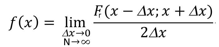
If an analytical function exists for f(x), this is the probability density function, which is also called probability distribution function, and is indicated with the symbol "pdf". If the probability density is integrated over the domain of X, from its lower extreme up to the considered value x, one obtains the probability that the random value is not higher than x, namely, the probability of not exceedance. The integral of the probability density can be computed for each value of X and is indicated as "cumulative probability". By integrating f(x), if the integral exists, one obtains the cumulative probability distribution F(X), which is often indicated with the symbol "CDF".

Figure 5. The probability function p(S) specifies the probability distribution for the sum S of counts from two dice. For example, the figure shows that p(11) = 1/18. p(S) allows the computation of probabilities of events such as P(S > 9) = 1/12 + 1/18 + 1/36 = 1/6, and all other probabilities in the distribution.
Example: the Gaussian or normal distribution The Gaussian or Normal distribution, although not much used for the direct modeling of hydrological variables, is a very interesting example of probability distribution. I am quoting from Wikipedia:
"In probability theory, the normal (or Gaussian) distribution is a very common continuous probability distribution. Normal distributions are important in statistics and are often used in the natural and social sciences to represent real-valued random variables whose distributions are not known [...] The normal distribution is useful because of the central limit theorem. In its most general form, under some conditions (which include finite variance), it states that averages of random variables independently drawn from independent distributions converge in distribution to the normal, that is, become normally distributed when the number of random variables is sufficiently large. Physical quantities that are expected to be the sum of many independent processes (such as measurement errors) often have distributions that are nearly normal. Moreover, many results and methods (such as propagation of uncertainty and least squares parameter fitting) can be derived analytically in explicit form when the relevant variables are normally distributed."
The probability density function of the Gaussian Distribution reads as (from Wikipedia):

where μ is the mean of the distribution and σ is its standard deviation.
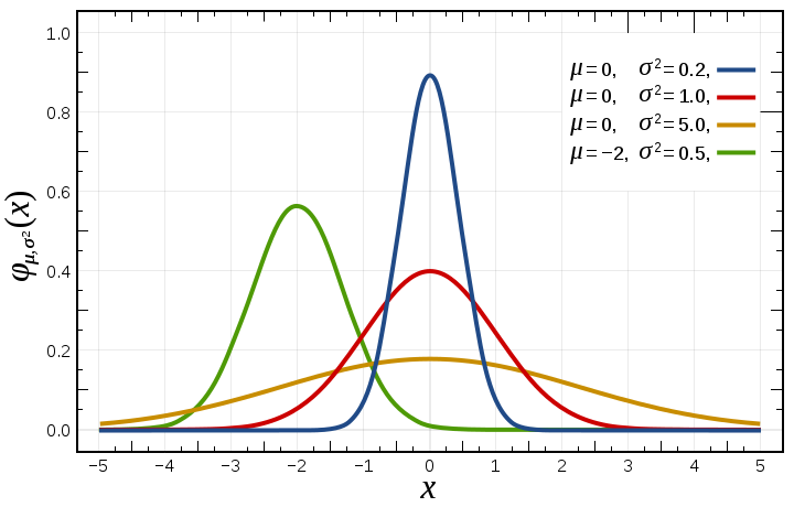
Figure 6. Probability density function for the normal distribution (from Wikipedia)
The above introduction to probability theory suggests the use of a widely applied method to estimate the peak river flow, that is, to estimate a probability distribution to describe the frequency of occurrence of peak flow data. In fact, we already realized that the return period, which is an essential information that conditions peak flow estimation, can be related to the frequency of occurrence and therefore the probability of occurrence. It follows that one can associate to a return period the corresponding probability of occurrence, which can be in turn related to the corresponding river flow through a suitable probability distribution. I will show below that this approach can be interpreted as a physically-based stochastic model. In fact, the return period is the inverse of the expected number of occurrences in a year. For example, a 10-year flood has a 1/10=0.1 or 10% chance of being exceeded in any one year and a 50-year flood has a 0.02 or 2% chance of being exceeded in any one year. Therefore, if we fix the return period we can derive the related peak flow by inverting its probability distribution. Furthermore, probability theory provides us with tools to infer the uncertainty of the estimate. For the sake of brevity we are not discussing how to estimate uncertainty when applying the annual maxima method.
In applied hydrology, the probability distribution of peak river flows is usually estimated by inferring the frequency of occurrence of annual maxima (see here for an example. Basically, from the available record of observations one extracts the annual maximum flow for each and the statistical inference is carried out over the sample of annual maxima. According to this procedure, the annual maximum return period is the average interval between years containing a flood of flow at least the assigned magnitude.
The annual maxima method is conditioned by the assumption that the random process governing the annual peak flow is independent and stationary. Independence means that each outcome of annual maximum flow is independent of the other outcomes. This assumption is generally satisfied in practice because it is unlikely that the occurrences of annual maxima are produced by dependent events (although dependence may happen if long term persistence is present, or the flood season crosses the months of December and January). Stationarity basically means that the frequency properties of the extreme flows do not change along time (please note that the rigorous definition of stationarity is given here.
Stationarity is much debated today, because several researchers question its validity in the presence of environmental change, and in particular climate change. In some publications the validity of concepts of probability and return period is questioned as well. However, the technical usefulness of stationarity as a working hypothesis is still unquestionable. For more information on the above debate on stationarity, see here and here.
Several different probability distributions can be used to infer the probability of the annual maximum flood. The most widely used is perhaps the Gumbel distribution, which reads as: F(x) = e-e-(x-μ)/β where μ is the mode, the median is  and the mean is given by
  where
where  is the Euler–Mascheroni constant
  The standard deviation of the Gumbel distribution is
  Once a sufficiently long record of river flow is available, the statistics of the distribution (i.e., the mean and the standard deviations) can be equated to the corresponding sample statistics and therefore the distribution parameters can be easily estimated.
The Gumbel distribution was proposed by Emil Julius Gumbel in 1958.
Example of application - Annual maxima method and Gumbel distribution Let us suppose that a record of 10 annual maxima is available, including the following observations (in m3/s): 239.0; 271.1; 370.0; 486.0; 384.0; 408.0; 148.0; 335.0; 315.0; 508.0 One is required to estimate the 5-year return period peak flow.
The mean of the observations is 346.41 m3/s and the standard deviation is 110.08 m3/s. Therefore, one obtains that β=85.80 and μ=296.88. The probability of not exceedance corresponding to the return period of 5 years is P(Q)=(T-1)/T=4/5=0.8 By inverting the Gumbel distribution one obtains: Q(T)= -β(log(-log(P(Q))))+μ or Q(T)= -β(log(log(T/(T-1))))+μ Therefore, one obtains: Q(5)=425.56 m3/s
1.3.1. Is the Gumbel distribution fitting the data well? When one applied a probability distribution to describe the frequency of occurrence of random events, the question should be raised on the capability of the probability distribution to provide a good fit. To check the reliability of the distribution, statistical tests can be applied. The most used test for verifying probability distributions is the Kolmogorov–Smirnov test. Please refer to the given link for a description of the test.

Figure 7. Illustration of the Kolmogorov–Smirnov statistic. Here, X is a generic random variable that can take both positive and negative values. Red line is CDF, blue line is an ECDF, and the black arrow is the K–S statistic (from Wikipedia. Please see the description of the Kolmogorov–Smirnov test on Wikipedia for mode details).
1.3.2. Data requirements for the annual maxima method The annual maxima method therefore requires the availability of a sufficiently long series of annual maxima. The larger the return period, the larger the sample size of the observed data should be. An empirical rule suggests not to extrapolate the Gumbel distribution beyond a return period that is twice the size of the observed sample. One should also take into account that the Gumbel distribution generally overestimates when extrapolated. A relevant question is where to find the data. Collecting hydrological data is very often a demanding task. For instance, in Italy there are several public offices collecting data and it is not always clear who is collecting what. The main reference in Italy is the former National Hydrographic Service, which has been absorbed by the Regional Agencies for Environmental Protection (ARPA). They use to publish the Hydrologic Annals, which report observations of river stage for several stations, and estimates of the related river flow for selected stations. An example of annal can be downloaded here.
1.3.3. Incorporating the physical basis The annual maxima method is essentially a purely probabilistic model, but actually it can be defined as a physically-based stochastic model where the physical knowledge is conveyed by the data. Indeed, the annual maxima deliver an extended set of information on the underlying physical processes leading to the formation of flood flows. However, the amount of physical information that is profited from by the annual maxima method is limited. Therefore, an interesting question is how to increase the physical basis, therefore gaining the means for deciphering the human impact. In order to identify the ways forward to get to target we need to better assess how the physical information conveyed by the data is exploited by the probabilistic analysis.
The information delivered by the data is employed by the annual maxima method through the estimation of the mean value E(X) and standard deviation σ(X of the random variable X which indicates the annual maximum flow. Through these statistics the parameters of the Gumbel distribution are estimated and the frequency of occurrence of the floods is subsequently inferred. Therefore, the key question that one needs to address is how to increase the amount of physical information that is used to estimate E(X) and σ(X. Increasing the physical basis is particularly valuable to reduce uncertainty when operating with data samples of limited size.
To reach the target, one may take profit from information on the contributing watershed, regional information, and rainfall-runoff models. These may allow the user to correct the estimates provided by the data for E(X) and σ(X. For instance, an additional estimate for E(X) may be delivered by regional relationship depending on the behaviours of the contributing catchment. Further details are provided in the lecture notes dedicated to the regional methods and rainfall-runoff models for peak flow estimation.
1.3.4. Alternative probability distributions for the annual maxima method There are several alternatives to the use of the Gumbel distribution within the annual maxima method. The most used probability distributions, besides the Gumbel, are the Frechet Distribution and the GEV distribution, which includes the Gumbel and Frechet distributions as special cases.
The annual maxima method presents the disadvantage of selecting and using for the statistical inference one value only per each year. Therefore, potentially significant events, occurred in the same year, may be discarded in the analysis. To resolve this problem, the peak-over-threshold method (POT) can be applied, which analyses all the peak values exceeding a given limit. Different probability distributions are usually applied to fit the obtained sample. More details are provided here.
The Generalized Pareto Distribution (GPD) is the most used probability model for threshold excesses and the shape parameter is determining the tail behavior of the distribution. Buoy measurements are the trustworthy data source and can be used in the analysis. The GPD distribution is characterized by three parameters: location, scale and shape. Location corresponds to the value of the threshold. If the shape and location are both zero, the GPD is equivalent to the exponential distribution. Packages are available in R to estimate the GPD parameters with several different estimators. More details on the GPD distribution are given here.
Various methods can be used for the threshold selection. There is a trade-off between bias of the estimated extreme design variables (low threshold) and variance due to the limited number of data used for estimating the GPD parameters (high threshold).
Mean residual life plot was suggested by Stansell (2004) to select the specific cut-off value. This graphical diagnostic technique is based on a characteristic property of the GPD distribution. In fact, if the GPD is a valid model for excesses over some threshold u0, then it is valid for excesses over all thresholds u > u0. Furthermore, for u > u0 it can be proved that the expected value of the difference given the given random variable and the threshold value, which can be estimated by the sample mean of the threshold excesses, is a linear function of u. This results provides a ready to use diagnostic technique which can be applied prior to the actual model fitting.
An alternative approach is to assess the stability of parameter estimates. Hence, this sensitivity analysis for model fitting is performed across a range of different threshold values. Finally, diagnostic checks can be applied once the GPD distribution has been estimated. They are not discussed here.
In many practical applications river flow data are not available at the river cross section of interest and therefore the annual maxima method cannot be applied. In such situations, one needs to apply estimation methods for ungauged catchments. These typically exploit alternative information, other than the data, on the hydrology of the considered catchment and river. A method that is frequently applied in the professional practice is to refer to a nearby gauged location, for which the peak river flow is estimated - perhaps using the annual maxima method - and then rescaled to the cross river section of interest by applying some similarity principle. For instance, one may assume that the unknown peak river flow Q(T) for the return period T is given by the relationship:
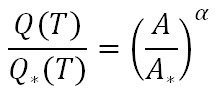
where Q* is the peak river flow in the gauged location, A and A* are the catchment areas for the ungauged and gauged locations, respectively, and α is an exponent for which the literature suggests the value of 1/3, which means that the specific contribution of the peak river flow (i.e., the peak river flow per unit catchment area) is increasing for decreasing extension of the contributing watershed.
1.4.1. The Index Flood method The concept of hydrologic similarity can be extended from one to several similar cross river sections, located inside a so called "homogeneous region". For all of them, it is assumed that the peak river flow Q(x,T) for the location x and return period T can be expressed through the relationship: Q(x,T) = i(x) F(T) where i(x) is the site-dependent mean annual flood, which is the average of the annual maxima, and F(T) is the regional frequency curve, which is invariant over the homogeneous region.
The regional frequency curve is estimated by fitting a suitable probability distribution to the sample of the specific peak flows (i.e., peak flow per unit catchment area) observed in the homogenous region, with the advantage that the sample size is larger with respect to the single site case. The index flood estimation is to be carried out over the considered site. It can be computed by averaging observed annual maxima, with the advantage that averaging entails less uncertainty with respect to extrapolating the estimation to large return periods through a probability distribution. In the absence of observed data, the index flood can be computed through regression techniques, depending on key features of the contributing catchment, which may include meteoclimatic and/or geomorphological behaviours.
Peak flow data may be extracted from a time series of flow values that are averaged over the observation time step. For instance, very often the river flow are observed at daily time scale, which means that the reading is taken at a certain hour during the day. The obtained observations are often regarded as average daily flow, from which the annual maxima (or the peak over threshold) can be selected. However, the peak flow is not coincident with the peak of the average daily flow. The latter is usually lower than the former, and the magnitude of the difference depends on the size of the basin, the time of concentration, the season, the meteoclimatic behaviours in general and so forth. Several empirical relationships have been proposed to estimate the ratio between annual maximum of the average daily flows and annual peak flow. See here for more details.
It was mentioned above that the processes that lead to the formation of flood flows are essentially physical processes, therefore obeying to Newton laws and conservation laws (mass, energy and momentum). These laws have not been explicitly used in the above described annual maxima method, although one may say, as I mentioned above, that these physical properties are implicitly resembled by the data.
In practical applications, one may wish to better profit from the above mentioned physical laws. In particular, when estimating the peak river flow one may experience situations where data scarcity makes the annual maxima method highly uncertain. Therefore, one may want to use additional information to reduce uncertainty. One possibility to reach the target is to make use of a rainfall-runoff model, which attempts to describe the rainfall-runoff transformation by making explicit or implicit use of the laws of physics. The rationale behind the application of a rainfall-runoff model is the attempt to reduce uncertainty by using information on rainfall over the catchment and additional information related to the catchment itself.
A rainfall-runoff model delivers an estimate of the river discharge at the catchment outlet depending on one or more input variables. At least one input variable, rainfall, is needed to feed the model, but other input variables may be used, like for instance temperature, wind speed, catchment topography and so forth. The model may deliver a point estimate of discharge, or a time series (a hydrograph). Analogously, it may require point estimates or time series of the input variables. Rainfall-runoff models are frequently used for estimating the peak river flow of flood hydrographs. We will focus on simple models by highlighting their physical basis and techniques for integrating them with probabilistic models to estimate their uncertainty.
1.6.1. The Rational Formula The Rational Formula delivers an estimate of the peak flow
it is dimensionally homogeneous and therefore one should measure rainfall in m/s and the catchment area in m2 to obtain an estimate of the river flow in m3/s.
A relevant question is related to the estimation of the rainfall intensity i to be plugged into the Rational Formula. It is intuitive that an extreme rainfall estimate should be used, which is related to its return period and the duration of the event. In fact, an empirical relationship, the depth-duration-frequency curve, is typically used to estimate extreme rainfall depending on duration and return period. When applying the Rational Formula, one usually assumes that the return period of rainfall and the consequent river flows are the same. This is assumption is clearly not reliable, but nevertheless is a convenient working hypothesis. Further explicit and implicit assumptions of the Rational Formula are listed below. As for the duration of the rainfall event, it can be proved, under certain assumptions, that the rainfall duration that causes the most severe response by the catchment, in terms of peak flow, is equivalent to the time of concentration of the catchment. It is important to note that the mean areal rainfall intensity over the catchment should be plugged into the rational formula. Therefore, for large catchments (above 10 km2 one should estimate i by referring to a central location in the catchment and an areal reduction factor should be applied.
The here (from https://ocw.camins.upc.edu/materials_guia/250144/2015/MetRacio1.pdf).
Singh (1992, p. 598) lists eight Rational Method assumptions (see also here). 1. “The computed discharge is the maximum that can occur for the selected rainfall intensity from that basin and that discharge occurs at the time of concentration and beyond.” 2. “The peak river flow is directly proportional to rainfall.” 3. “The frequency of the peak discharge is the same as the frequency of rainfall" (see above). 4. “The relation between peak discharge and the drainage area is the same as the relations between peak discharge, intensity, and duration of rainfall. This means that the drainage basin is considered linear.” 5. “The coefficient of runoff, C, is the same for storms of various frequencies". This means that all the losses on the drainage basin are a constant. 6. “The coefficient of runoff is the same for all storms on the drainage basin regardless of antecedent moisture condition". 7. “Rainfall remains constant over the entire watershed during the time of concentration". The significance of this assumption is that because of the spatial variability of rainfall, the drainage area for which the rational method will apply is limited. 8. “Runoff occurs nearly uniformly from all parts of the watershed". This means that the runoff coefficient must be nearly the same over the entire drainage basin. This assumption is less likely to be valid as the drainage-basin size increases.
Although very simple, the Rational Formula is extremely useful in hydrology to increase the physical basis when estimating peak flow and to get baseline estimates.
The estimation of the flood hydrograph can be carried out through rainfall-runoff models simulating an entire event or an extended series of data. These models will be described in the lecture dedicated to rainfall-runoff modeling.
A simpler approach is to estimate the flood volume by using probabilistic models, like for instance a bivariate probability distribution of peak flow and related hydrograph volume. Once the volume is estimated, one may assume a predetermined form for the flood hydrograph, like for example the triangular symmetric shape, therefore easily obtaining the full definition of the extreme hydrograph for a given return period. One should consider that the return period of the peak flow is generally different with respect to the return period of the corresponding flow volume. An interesting treatment of the problem is reported here.
Stansell, P. (2004). Distributions of freak wave heights measured in the North Sea. Applied Ocean Research, 26(1), 35-48.
Last updated on May 7, 2017
- 90 views