

Harbor basins and ports are often protected with structures like breakwaters to mitigate the impact of waves and currents therefore creating a sheltered environment to facilitate the approach of ships and mooring operations. A side effect that often arises is the deposition of sediments due to lowering the energy of the marine environment inside the harbor with respect to the immediate outside. In fact, siltation is often experienced when a low energy environment is located in the proximity of a high energy one that has the capability to mobilise the sediments themselves. Siltation reduces the sea depth and may originate obstruction of the port traffic (see Figure 1).
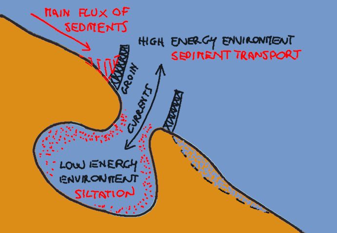
Figure 1. Dynamics of sediments in low energy environment
Siltation rates vary depending on the characteristics of the harbour and the marine environment. To give an example, volumes of sediments up to 3.5 millions of cubic meters per year (with a tickness up to more than one meter) have been observed in the Botlek New Waterway, in Rotterdam. Siltation rates in particular depend on:
- distance from open sea;
- area of the harbour basin;
- area of the entrance in the basin;
- tidal range and duration;
- peak tidal current outside the entrance;
- outside concentration of sediments;
- density difference inside and outside the basin.
Harbour siltation is higher (factors up to the value of 5 have been observed) in salt and brackish water conditions than in fresh water conditions (van Rijn, 2016), for the higher concentration of sediment and the generation of stratified flow in the presence of salt water. An issue related to harbour siltation is the degree of contamination of the deposited sediments and mud, which is impacting the dredging procedures and costs. Contamination may be due to local or non-local sources.
To maintain the functionality of ports in the presence of significant siltation it is often necessary to perform harbor clearance works through dredging. Dredging is the removal of sediments and mud from the bottom of water bodies. The material resulting from dredging may be used for beach replenishment or other forms of recycling. Dredging may be carried out by using a set of techniques that are characterised by different operational modes and impact on the port activity and the environment in general. Planning and managing dredging activities are essential tasks to port operation and maintenance, that are regulated by prescriptions and technical guidelines issued by national and local administrations and port authorities.
The dynamics of sediments, which leads to their transport and deposition, can be analysed by using models which may allow to draw predictions and planning of dredging operations. Models can also be used to study the impact of sediment removal, which may cause turbidity and concentration of sediments elsewhere.
Different type of models can be used. Laboratory small scale models can be set up at an appropriate scale (micro, small, medium and large scale models). These are also termed "physical models". Numerical models make use of computer codes to apply equations that are typically physically-based. Given that fluid dynamics is governed by the fundamental laws of physics candidate equations are conservation laws, like conservation of mass, conservation of energy and momentum. Composite models refer to the integrated and balanced use of physical and numerical models.
Physical models and laboratory experiments are frequently used to model sediment dynamics in coastal areas. They present the relevant advantage of allowing repeatable experiments and allow to reproduce highly heterogeneous, turbulent and 3-dimensional processes. However, their scale cannot be too small, as the effect of viscosity may prevail over turbulence if the prototype is compressed to a small size. Therefore, large facilities are typically needed to apply physical models of large harbors.
The fulfillment of appropriate similarity criteria is a necessary condition for the physical model to provide a reliable reproduction of the reality. Ensuring similarity often implies modeling requirements that are not easy to satisfy. The scientific literature in this regard is particularly ample, and summarizes an experience that is now more than one century old. Physical models are normally required on the one hand to represent the relevant phenomena with sufficient reliability and on the other hand to convince the designer and the stakeholders of the reliability of the results they provide. In relation to the first aim, it is essential to emphasize the term "relevant phenomena". In fact, it is often not possible to fully reproduce fluid mechanics within a small scale physical model. Therefore, it is essential to identify priorities for the modelling purpose and to make sure that the relevant phenomena for that purpose are reproduced with sufficient approximation. In relation to the second purpose, however, it is necessary that the correspondence between the real phenomena and those reproduced in the model is simple and as complete as possible, easily perceptible in relation to the similarity of models with reality and the care in the representation. Oversimplification of details may lead to lack of confidence in the results by the stakeholders.
To understand similarity, let us make a simple premise: to reproduce the reality (prototype) in a small scale model implies a change in physical quantities that is equivalent to what is obtained if we changed the geometric units of measurement. In fact, the measurement of a physical quantity is defined as the ratio between the same quantity and another of the same type (such for instance a length) that is taken as a unit of measurement. As this unit of measurement varies, all the measurements under consideration change as well, precisely as in a small scale model; the relationship between the measurements of two quantities of the same type, on the other hand, remains unchanged, and therefore assumes an objective value, which is valid for both model and reality.
Experimental evidence has shown that there are rigorous links between the measurements of quantities of different type, which are expressed by physical laws. For instance, of we change the unit of measurement of length, then the measure of velocity will also change. Therefore, we may divide the physical quantities into fundamental quantities, for which it is necessary to define the units of measurement, and derived quantities, whose unit of measurement can instead be inferred from the units of the fundamental quantities by means of the aforementioned physical laws. Similarly, if we change the geometric size of a real system then derived quantities will change according to the above laws.
The number and nature of the quantities for which it is necessary to define the unit of measurement, and therefore to be considered as fundamental, is arbitrary, but the quantities must be dimensionally independent. Classical mechanics is governed by three fundamental quantities which conventionally are length, whose unit of measurement will be indicated below with the symbol L, time (T) and mass (M). The units of measurement of the fundamental quantities are established by conventions. However, it is in principle possible to adopt new units for mass, length and time, say for instance and respectively, rM, rL, rT. As a result of the above change, the units of measurement of the derived quantities will also be different. The new unit for the derived quantity A will have measure rA with respect to the previous unit of A, and this value will depend on the changes imposed on the fundamental units, that is
rA = f(rM, rL, rT) (1)
The nature of the functional relation f is constrained by the need to define the measures so as to preserve the value of the relations between quantities of the same type which, as we mentioned, above, have an objective value. It can be shown that this condition is satisfied if and only if f takes the form of a product of powers, so that (1) becomes
![]() (2)
(2)
The exponents αA, βA and γA are determined by the functional relationship that relates A to the fundamental quantities length, time and mass. For instace, if A was velocity v, which is obtained by dividing length by time, then βA=1 and γA=-1.
If αA, βA and γA are equal to zero, the unit of A does not change even if the fundamental units are changed and then we say that A is a dimensionless quantity, namely, a pure number. Conversely, if only αA and γA are equal to zero, then we say that A is geometric quantity, while if only αA is equal to zero then we say that A is a kinematic quantity. Dynamical quantities are instead characterised by nonzero values of all the exponents.
Therefore, changes of the measure units of the three fundamental quantities imply rigorously defined changes of the derived quantities. Conversely, a new choice for the units of three derived quantities that are dimensionally independent implies a consequential change of the units of the fundamental quantities.
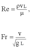
In the case of fluid mechanics, the mass density of the fluid ρ, the speed v, and the length L, which are three dimensionally independent quantities, are often assumed as fundamental quantities. On the other hand, we can prove that fluid mechanics phenomena can be fully described, in the absence of thermodynamic, electromagnetic and chemical effects, by 9 quantities, i.e. length, time, speed, acceleration of gravity, pressure, mass density of the fluid, dynamic viscosity, compressibility and surface tension. Since 3 of these quantities are fundamental, the remaining 6 can be expressed in terms of dimensionless ratios between the fundamental quantities, or 6 pure numbers. They are the Reynolds, Froude, Weber, Mach, Euler, Strouhal numbers. These numbers, being dimensionless, must necessarily assume the same value in the model and in the reality.
All these pure numbers, with the exception of Strouhal's, can be interpreted, from the dynamic point of view, as the ratio between the force of inertia, expressed by the term ρ L2v2, where L is a characteristic length of the fluid flow (like pipe diameter for pipe flow, the hydraulic radius for the open channel flow and so forth), and the forces of a different nature each time acting on an assigned volume of fluid. For example, the Reynolds number can be expressed as the ratio between the force of inertia and the force of viscous friction, expressed by the term μLv, so that it results Re=(ρL2v2)/(μLv)=ρLv/μ. The Froude number can instead be obtained by setting the force of gravity as denominator, expressed by the term ρL3g, so that we have Fr2=ρ (L2v2)/(ρL3g)=v2/(gL). Some of these numbers also have a kinematic interpretation: for example, the Froude number can be interpreted as the ratio between the velocity of the fluid and the velocity of propagation of a gravitational wave of small amplitude, while the Mach number can be expressed as the ratio between the velocity of the fluid and the velocity of propagation of an elastic perturbation.
While the number of quantities to fully describe a fluid mechanics process is 9, one has to take into account that some of these quantities may have a negligible or null role in describing specific processes and therefore can be dropped. On the other hand, if additional processes are to be described, such as sediment transport in our case, then one needs to consider additional quantities like for instance the diameter and the mass density of the sediments, which in turn lead to identifying the particle Reynolds number and the densimetric Froude number as additional pure numbers.
The validity for the prototype of the observations made on the model is ensured by the respect of the similarity laws, which can be respected even when the fluids used in the model and the reality are different. This can be an advantage in some cases; for example when it comes to studying the motion of particular fluids, such as oil or inflammable substances, which can be replaced in the model by fluids that are easier to use or simply cheaper, such as water or air.
By modifying the units of measurement of the fundamental quantities, which we now suppose to be length L, mass M and time T, it is possible to adopt other units having measure λL, λM and λ T with respect to their respective original units, namely
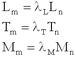 (3)
(3)
where the subscript n and m refer to the measurements taken with the previous and new units, respectively.
Basing on the conversion scale of the fundamental units given by (3) one can derive the scale of any derived measure. For instance, for the generic quantity A one can write
![]() (4)
(4)
where αA, βA and γA are the exponents introduced into (2).
Given that the same physical laws apply to both model and reality, one may simply say that in a small-scale model the measurement of the involved quantities are changed according to the involved physical laws, so that they take measurements respectively λL, λM and λT with respect to the original sizes in the reality. The choice of λL, λM and λT cannot be arbitrary, as the pure numbers must remain unchanged, thus ensuring the validity for the model of all the physical laws referring to the reality. This consideration suggests the idea that a mechanical phenomenon can be studied in an artificial "small world" which is the reduced-scale model, in which lengths, masses and times are reduced according to the reduction scales respectively λL, λM and λT suitably selected.
One easily realizes that it would be impossible to ensure the conservation of all P independent pure numbers that characterize a phenomenon, unless a unique reduction ratio is used which is given by the characteristics of the fluids and the acceleration of gravity in the two environments. Since the latter is almost constant and, at least in hydrodynamics models, the same fluid is almost always used (namely, water), it is found that the conservation of pure numbers, that is the perfect dynamic similarity between model and prototype, can only be obtained if the scale of geometric reduction is 1:1. That is, the only model in perfect dynamic similarity with the reality is the reality itself.
The above assertion can be proved by reductio ad absurdum. Accordingly, let us assume that a model in which a marine current is reproduced in an environment characterized by an acceleration of gravity equal to g, is able to simultaneously ensure the conservation of the Reynolds and Froude numbers, which are expressed in the form
 (5)
(5)
which leads to
 (6)
(6)
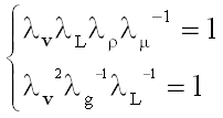
namely
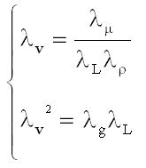 . (7)
. (7)
Given that λg, λρ e λμ assume unit value since gravity and the fluid (water) are unchanged, one obtains,
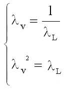 , (8)
, (8)
which of course gives incompatible conditions.
We conclude that it is not possible to have a small scale marine model that is perfectly similar to the prototype and it is necessary to accept models that are only partially similar, that is, for which the conditions of similarity are respected with reference not to all but only to some of the acting forces. In practice, it is necessary to make assumptions, that is, to identify which are the dominant forces on the phenomenon and to keep only these in conditions of similarity with each other. In most models of marine currents these may be the Froude number and/or the Reynolds number.
It follows that large scale models are desirable since in this way the values of Froude and Reynolds number do not change much. For wave reproduction the capillary forces should play an insignificant role. Consequently, the wave lengths must not be too short. Very small scales also affect the repeatability by which the small scale waves can be reproduced in the laboratory. In tests where viscous effects are important, attention has to be paid to the Reynolds number. This is related primarily to the coastal structure being tested rather than to the ability to reproduce the waves. However, micro-models can be used as a tool for preliminary research, the development and initial testing of novel ideas, the preliminary design of wave related coastal protection schemes and the testing of alternative design options, the provision of immediate answers and insights to simple coastal engineering problems, the pre-design of large scale physical models (see also http://www.coastalwiki.org/wiki/Modelling_coastal_hydrodynamics). More details on physical models can be found here (in Italian).
The increasing availability of computing power in the last three decades has stimulated the use of numerical models to study sediment hydrodynamics within harbours and ports. Computer models exhibit the advantage of easy applicability even to large scale domains with a relatively low cost in terms of human resources and required facilities. They are limited by the assumptions underlying their representation of coastal hydrodynamics and morphodynamics which needs adequate consideration. Any modelling applications is affected by uncertainty and numerical models do not make an exception, but the nature of their uncertainty is different with respect to physical models. Several models have been proposed to study coastal sediment transport. They make use of finite elements, finite differences, boundary elements, finite volumes with both an Eulerian or a Lagrangian approach. The numerical algorithm can be implicit, semi-implicit, explicit, or characteristic-based. The modelling can be simplified by using a one-dimensional (1D) representation model, as well as two-dimensional (2D) and three-dimensional (3D) ones. Their accuracy depends on the adopted scheme, their numerical stability, the quality of the underlying information, the initial and boundary conditions and so forth. Application of numerical models requires a consolidated experience and - perhaps more important - a mature knowledge of the problem at hand, its inherent natural processes and the model theory. A careful assessment of the reliability of the model results is always needed for the purpose of applied design of sediment management. Such assessment cannot be carried out without a full understanding of the underlying theory and a good perception of the modelled processes and their dynamics. It should be also considered that the communication between the modelers and the users is more challenging when presenting the results of numerical models which maybe difficult to understand. The recent development of high level visualisation tools may allow the mitigare this latter problem (see Figure 2).
Figure 2. Faster than real-time simulation with the Boussinesq module of Celeris, showing wave breaking and refraction near the beach. The model provides an interactive environment. By Sasan Tavakkol, CC BY-SA 4.0
We have mentioned above that physical and numerical models rely on different assumptions and therefore are affected by different types of uncertainty. The latter evidence suggests the idea to combine the two different types of models to reciprocally compensate their uncertainties. The combination of approaches requires the availability of relevant resources, expertise and facilities and is therefore used for studying important problems. It is an increasingly used approach which may allow one to make an optimal use of the available information.
Sediment hydrodynamics and morphodynamics can als obe studied with empirical and heuristic approaches which are useful for obtaining a first approximated solution, which may be useful for preliminary design. An example of a simple 1-D numerical model, which can be considered an heuristic approach in consideration of its very simplifying assumption, is the one-line model that is described here. The literature also proposes examples of zero-dimensional models that treat a given harbour as a tank, like for instance the approach proposed by Eysink (1989). Figure 3 presents a sketch of a modified version of the latter model.
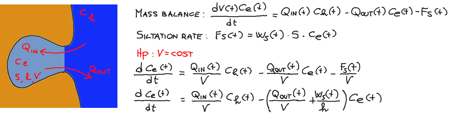
Figure 3. Skectch of a zero-dimension model of harbour siltation.
In Figure 3, S, h and V indicate the projected area, depth and volume of the harbour basin, respectively. QIN and QOUT indicate the time varying inflow and outflow from the basin, respectively, Ce and Ch indicate the concentration of sediments inside and outside the basin, respectively, Fs is the time varying siltation rate and Ws is the effective siltation velocity. It is assumed that changes of V are negligible and therefore V can be assumed to be constant (and is indeed constant if QIN=QOUT at each time step). In steady state such model tends to an equilibrium configuration that depends on Ws and gives assigned siltation rates. In unsteady state conditions the model lends itself to a numerical solution.
Another example of empirical model is the semi-empirical box method (van Rijn, 2016).
Monitoring of the siltation processes is an essential step to plan dredging operations, as well as the assessment of the context and its environmental behaviours, including mud contamination.
Planning of dredging operations has to be supported by a comprehensive monitoring program to assess dredging effectiveness and to ensure compliance with guidelines and regulations. Monitoring should include:
- Assessment of the bathymetry of the dredged area during inter-dredging periods, to quantify dredging effectiveness. Bathymetry data are compared with volumes of sediment removal to gauge removal effectiveness. Evaluation of the thickness of the dredged residuals allows to monitor progress toward achieving cleanup levels and to determine the need for additional dredging.
- Measurement of contaminant concentration. Pre- and post-dredging contaminant concentrations may be compared to understand dredging impacts to the environment. Contaminant concentration may be evaluated by taking samples of sediments.
- Measurement of total suspended solids or turbidity in the dredge area and downstream to monitor resuspension and transport of sediment and contaminants and evaluate compliance with standards. These measurements can e taken by sampling the water column or by installing and operating continuous real-time measurement probes.
- Air and water quality to ensure compliance with state and other standards if contaminants are released in the atmosphere and surrounding waters.
- Wind and Current to monitor to predict flow conditions during dredging operations.
Monitoring is also useful to assess whether the targets of the designed dredging have been met and to provide technical and administrative reports to the relevant authorities.
Dredging is a potentially risky operation that must be supported by adequate planning. Administrative and regulatory requirement are essential constraints that one should take into account during the planning process. To provide an example, in Italy dredging is not allowed in the marine archeological sites, in the areas with relevant biological and ecological value, in the zones of repopulation, in the proximity of coastal areas with relevant environmental value, in the presence of underwater cables and pipes and other areas that are specified by local and national regulations. Furthermore, it is prescribed to minimise the environmental impact through:
- minimising the water content of the removed material;
- minimising the dispersed material;
- limiting water turbidity and the mobilisation of pollutants;
basing on detailed information on:
- preliminary classification of the material to be dredged.
Planning should be first based on predictions of siltation, obtained through suitable models by taking into account the required clearances for ship's approach. Predictions allow to estimate the periodicity of dredging, to be verified through monitoring.
Furtermore, a detailed assessment of the environmental impact should be carried out by referring to:
- local bathymetry and its changes;
- increase of local turbidity during dredging and its effect on the environmental quality of the neighbouring areas;
- possible diffusion of contaminants in the water column;
Transportation of the dredged material on land when needed, and its disposal should also be adequately considered.
Dredging mud disposal is an emerging problem for several harbours, which needs to be planned basing on mud characterisation. If the sediments are clean they can be used for landfilling (land reclamation) or beach replenishment. However, muds are often contaminated. The management of contaminated sediments is a significant concern today. Because of a variety of maintenance activities, thousands of tonnes of contaminated sediment are dredged worldwide from commercial ports and other aquatic areas. Several case studies of reuse of dredged material are presented web site of the Central Dredging Association. An example of reuse of contaminated muds is presented here.
A schematic representation of the workflow for mud treatment and disposal is given in Figure 4.
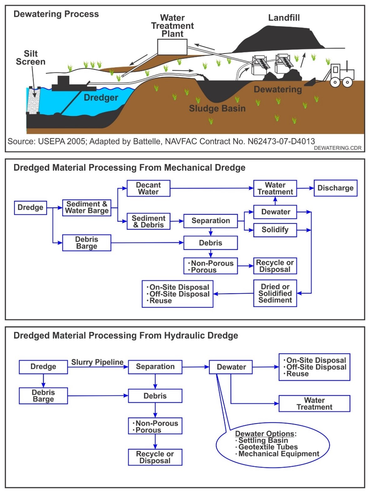
Figure 4. Schematic of mud treatment disposal processes (from https://frtr.gov/matrix/Dredged-Material-Processing-Technologies/).
Mud characterisation should determine the following parameters (van Rijn, 2019):
- in-situ wet bulk density over the depth of the deposits (bulk density profile);
- sediment composition in terms of fraction clay/lutum< 4 μm; fraction silt 4 to 63 μm; fraction fine sand> 63 μ;
- settling velocity;
- consolidation parameters;
- critical shear stress for erosion;
- yield stress and flow point stress.
Wet bulk density is an important parameter that may condition to treatment of the mud. The dry density of sediments can be expressed as a function of porosity, defined as the volume of voids per unit volume of the mixture, namely:
η = Vv/(Vv + Vs),
where Vv is volume of voids and Vs is the volume of solids, e.g., Vv+Vs is the total volume of the mud. Porosity is related to the dry density of the mixture through the relationship ρd,m = ρs(1-η) where ρs is sediment density. Porosity is related to the amount of water contained in the mud, which one generally needs to extract before disposing the mud itself. In fact, landfill sites are today decreasing in number and therefore a reduction of the volume of dredged sediment through dewatering is often a necessary operation to ensure the sustainability of dredging in the future.
There are two types of dewatering methods: passive and mechanical. In addition, solidification is commonly used as a sediment dewatering method. Treatment of the separated water may be required prior to return to the waterbody. The need for treatment will depend on level of contaminants and local regulations.
An interesting treatment of the main issues related to sediment disposal is given by the web site of the Federal Remediation technologies round table.
Dredging techniques can be broadly divided into three categories:
- suction dredging;
- mechanical dredging;
- water injection dredging.
Suction dredging is operated by using a simple suction at the open end of a suction pipe that is covered by a grid to avoid the entrance of large objects that may obstruct the pipe itself. It is a technique that is recommended for for sand extraction rather than the removal of consolidated layers. The soil may be loosened by the eddies of water flow only, with no other mechanical action, or the suction head can be equipped with a cutting mechanism at the inlet (in this case some textbooks classify this technique as mechanical dredging). By moving the suction tube at a proper speed, a continuous removal of sediments can be attained. See Figure 5 for a schematic of suction dredging and Figure 6 for an example of suction dredge barge.
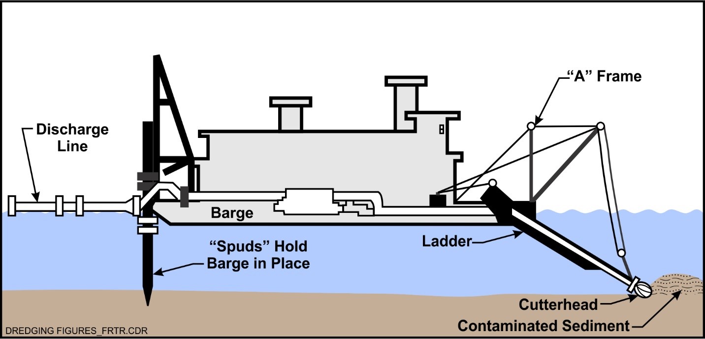
Figure 5. Schematic of suction dredge (from https://frtr.gov/matrix/Environmental-Dredging/).
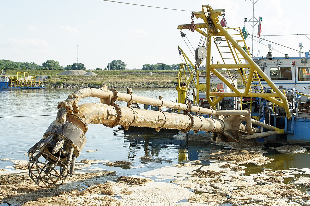
Figure 6. The dredge drag head of a suction dredge barge on the Vistula River, Warsaw, Poland. By Dariusz Kowalczyk, CC BY-SA 4.0, https://commons.wikimedia.org/w/index.php?curid=49880395
Mechanical dredging makes use of mechanical tools to loosen the soil and lift the sediments at the land level. It typically involves the use of an excavator or another type of heavy equipment, that is usually placed on a barge or on the water's edge, to excavate out the sediments which are then carried away for disposal or reuse. From the site of the Federal remediation technology round table one reads:
Mechanical dredges use digging buckets such as a clamshell suspended by a cable from a crane, an excavator on a fixed arm, or dragline buckets suspended by a cable from a crane. Mechanical dredges remove sediment with a similar density and water content as the in-place material. Some water is added to the sediment because the clamshell and bucket are not always completely full of sediment. Mechanical dredges typically add a water volume that is 0.2 to 0.5 times the in-place sediment volume. Some sediment also is released into the water column as the bucket is raised. Environmental dredging buckets, having specially designed seals, often are employed to minimize release of sediment during dredging.
See Figure 7 for a schematic of mechanical dredge.
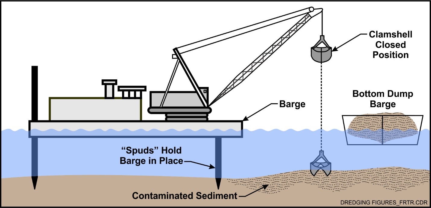
Figure 7. Schematic of mechanical dredge (from https://frtr.gov/matrix/Environmental-Dredging/).
See also Figure 8 for a schematic of bucket dredging while Figure 9 show grab clamshell dredging in progress.
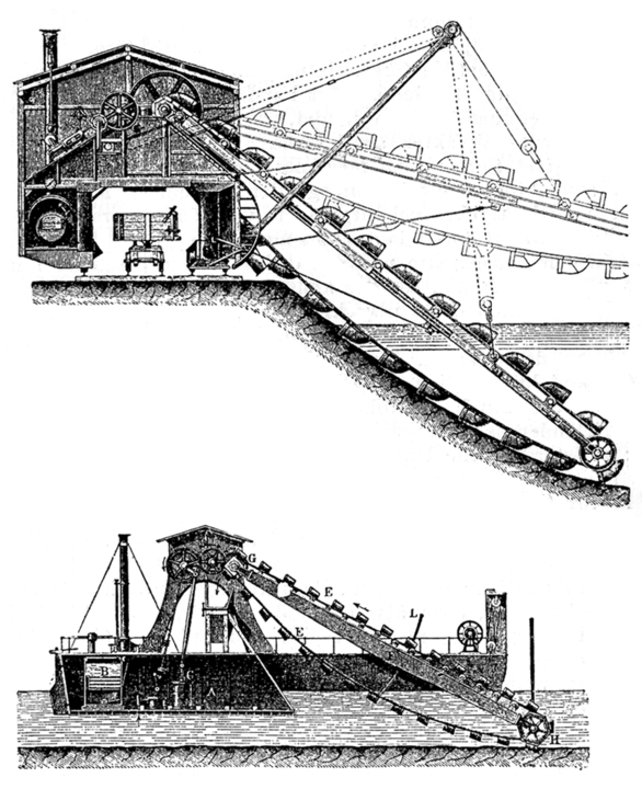
Figure 8. Schematic of bucket dredging. Public Domain, https://commons.wikimedia.org/w/index.php?curid=1038410.
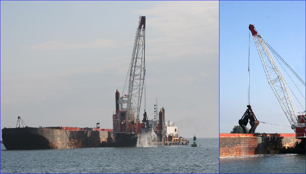
Figure 9. Grab (clamshell) dredging in process in Port Canaveral, Florida. CC BY 3.0, https://en.wikipedia.org/w/index.php?curid=14370430.
Figure 10 shows a schematic of the famous cutter suction dredger called "Mashhour" operated by the Suez Canal Authority in Egypt. When it was first launched in 1996 it was said to be the largest and most powerful cutter suction dredger of its kind in the world, and was designed to dredge abrasive sand with gravel, compacted sand, sticky clay and rocks in the widening and deepening of the Suez Canal to allow even larger ships to pass. Its numbers are impressive: the total installed power is 22795 kW, the length of the hull and length overall are 113.40 m and 140.30 m respectively, the width is 22.40 m, the maximum draught is 7.20 m, the maximal dredging depth is 35 m, the cutter power is 3000 kW, the diameters of suction pipe and discharge pipe are 1000 mm and 850 mm, respectively. The Mashhour was used to clear the Suez Canal after the blockage that occurred at the end of March, 2021.
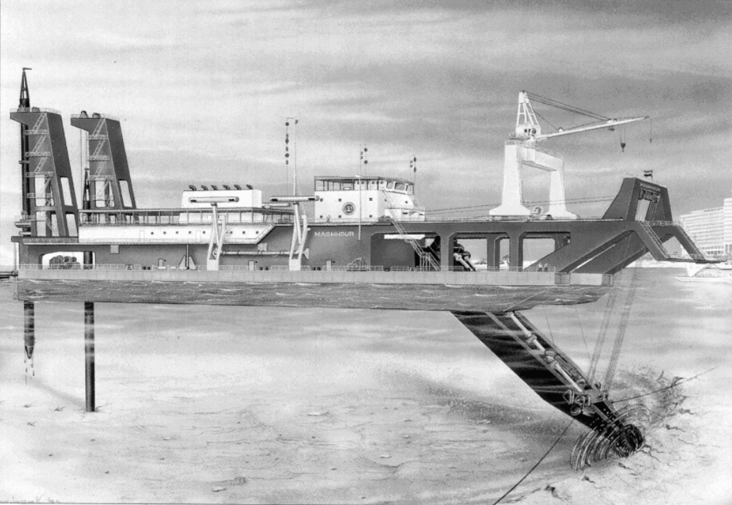
Figure 10. Mashhour, one of the biggest cutter suction dredger today operational.
Water injection dredging is a relatively new dredging technique. A water injection dredger uses a small jet to inject water under low pressure (to prevent turbidity relevant increase in the surrounding waters) into the soil layer to fluidise it and originate a turbidity current. The jet nozzles are mounted on a horizontal tube that has a length between 4 and 15 meters. The mobilized sediments then flow away downslope along the sea bottom for the effect of gravity, natural or artificially induced currents and sediment concentration gradient. The dredge has to keep moving to avoid low densities of the water-soil mixture, which may results in the dispersion of the mixture along the whole water column. In fact, the aim of water injection dredging is to move material horizontally in the vicinity of the seabottom. To reach the latter target, two conditions have to be met:
- First, it is necessary to mobilize and maintain a high-velocity and high-concentration flow of mud. This implies that the densimetric Froude number of the mud flow should be larger than 1 (supercritical mud flow). The Froude number of the mud flow is given by
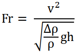 (9)
(9)with v being the mud flow velocity, h the tickness of the mud flow layer, ρ the mud density and ∆ρ = (ρ-ρw) = (ρs-ρw)c where ρs is mass density of sediments, ρw is mass density of sea water and c is concentration of sediments into the mud.
- Second, the high concentration mud layer should be stable. Its stability depends on the local Richardson number defined as
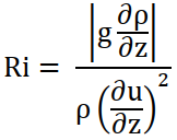 (10)
(10)where z indicates the coordinate along the vertical direction and the derivative of the mud density can be given by the density gradient between the mud and fresh water. The Richardson number is the ratio between the stabilizing effects of gravity and density gradient and the destabilizing effect of the near-bed velocity gradient (Mastbergen and Van den Berg, 2003; van Rijn, 2015). Experimental research shows that the high concentration mud layer is stable for Ri>0.25.
Water injection can be applied to a limited variety of soil types only, like silts, unconsolidated clays and fine sands. It is not efficient for plastic clays and consolidated material in general.
A significant advantage of water injection dredging is that sediments disposal occurs naturally along the seabed as the sediments are not raised at the surface. This process occurs with a minimum of disturbance to the equilibrium of the ecosystem. With water injection dredging nature takes care of the sediment transport, making water injection dredging under certain conditions a very environmentally friendly cost-efficient dredging technique.
This video illustrates how water injection dredging works.
Dreadging is an important operation for port management and maintenance. It should be based on the understanding of local marine conditions and sediment dynamics, monitoring and an efficient plan for dredging activities, mud characterisation, treatment and disposal. In particular, mud disposal is today an emerging issue in view of its potential environmental impact. This lecture provides a brief overview of the subject. Extended additional information is given by the references below.
Mastbergen, D.R. and Van den Berg, J.H., 2003. Breaching in fine sands and the generation of sustained turbidity currents in submarine canyons. Sedimentology, Vol. 50, 625-637
van Rijn, L.C. (2016). Harbour siltation and control measures, available for donload at http://www.leovanrijn-sediment.com/
van Rijn, L.C. (2015). Water injection dredging, available for donload at http://www.leovanrijn-sediment.com/
van Rijn, L.C. (2019). Land reclamation of dredged mud; consolidation of soft soils, available for donload at http://www.leovanrijn-sediment.com/
Vlasblom, W., University lecture notes, 2003, Delft University of Technology, available at https://www.dredging.org/dredging-equipment-and-technology/53
http://www.leovanrijn-sediment.com/ http://www.coastalwiki.org/wiki/Modelling_coastal_hydrodynamics https://frtr.gov/matrix/Environmental-Dredging/ https://www.dredging.org/dredging-equipment-and-technology/53
Last modified on April 13, 2021
- 252 views