
Deductive assessment of water resources availability is carried out by applying mathematical models which simulate the water flow in the surface river network or underground aquifers. Modeling of surface water is usually carried out through hydraulic models or rainfall-runoff models. Aquifers are modeled by applying groundwater models.
Rainfall-Runoff modeling is one of the most classical applications of hydrology. It has the purpose of simulating a river flow hydrograph in a given cross river section induced by an observed or a hypothetical rainfall forcing. Rainfall-runoff models may include other input variables, like temperature, information on the catchment or others. Within the context of this subject, we are studying rainfall-runoff models with the purpose of producing simulation of long term hydrographs. Rainfall-runoff modelling is a cross cutting topic over several of the major issue this subject is focusing on.
Rainfall-runoff models describe a portion of the water cycle (see Figure 1) and therefore the movement of a fluid - water - and therefore they are explicitly or implicitly based on the laws of physics, and in particular on the principles of conservation of mass, conservation of energy and conservation of momentum. Such conservation laws apply to a control volume which includes the catchment and its underground where water flow takes place. The catchment is defined as the portion of land whose runoff uniquely contributes to the river flow at its closure river cross section.
Depending on their complexity, rainfall-runoff models can also simulate the dynamics of water quality, ecosystems, and other dynamical systems related to water, therefore embedding laws of chemistry, ecology, social sciences and so forth.
Models are built by constitutive equations, namely, mathematical formulations of the above laws, whose number depends on the number of variables to be simulated. The latter are the output variables, and the state variables, which one may need to introduce to describe the state of the system. Constitutive equations may include parameters: they are numeric factors in the model equations that can assume different values therefore making the model flexible. In order to apply the model, parameters needs to be estimated (or calibrated, or optimized, and we say that the model is calibrated, parameterized, optimized). Parameters usually assume fixed value, but in some models they may depend on time, or the state of the system.

Figure 1. The hydrologic cycle (from Wikipedia)
Rainfall-runoff models can be classified within several different categories. They can distinguished between event-based and continuous-simulation models, black-box versus conceptual versus process based (or physically based) models, lumped versus distributed models, and several others. It is important to note that the above classifications are not rigid - sometimes a model cannot be unequivocally assigned to one category. We will treat rainfall-runoff models by taking into consideration models of increasing complexity.
The Rational Formula delivers an estimate of the river flow
it is dimensionally homogeneous and therefore one should measure rainfall in m/s and the catchment area in m2 to obtain an estimate of the river flow in m3/s.
A relevant question is related to the estimation of the rainfall intensity i to be plugged into the Rational Formula. It is intuitive that an extreme rainfall estimate should be used, which is related to its return period and the duration of the event. The return period is defined as the average time lapse between two consecutive events with rainfall intensity reaching or exceeding a given threshold. In fact, an empirical relationship, the depth-duration-frequency curve, is typically used to estimate extreme rainfall depending on duration and return period. When applying the Rational Formula, one usually assumes that the return period of rainfall and the consequent river flows are the same. This is assumption is clearly not reliable, but nevertheless is a convenient working hypothesis. Further explicit and implicit assumptions of the Rational Formula are listed below. As for the duration of the rainfall event, it can be proved, under certain assumptions, that the rainfall duration that causes the most severe response by the catchment, in terms of peak flow, is equivalent to the time of concentration of the catchment. It is important to note that the mean areal rainfall intensity over the catchment should be plugged into the rational formula. Therefore, for large catchments (above 10 km2 one should estimate i by referring to a central location in the catchment and an areal reduction factor should be applied.
The here (from https://ocw.camins.upc.edu/materials_guia/250144/2015/MetRacio1.pdf).
Singh (1992, p. 598) lists eight Rational Method assumptions (see also here). 1. “The computed discharge is the maximum that can occur for the selected rainfall intensity from that basin and that discharge occurs at the time of concentration and beyond.” 2. “The peak river flow is directly proportional to rainfall.” 3. “The frequency of the peak discharge is the same as the frequency of rainfall" (see above). 4. “...the drainage basin is considered linear”, namely, the rainfall-runoff relationship is linear. 5. “The coefficient of runoff, C, is the same for storms of various frequencies". This means that all the losses on the drainage basin are a constant. 6. “The coefficient of runoff is the same for all storms on the drainage basin regardless of antecedent moisture condition". 7. “Rainfall remains constant over the entire watershed during the time of concentration". The significance of this assumption is that because of the spatial variability of rainfall, the drainage area for which the rational method will apply is limited. 8. “Runoff occurs nearly uniformly from all parts of the watershed". This means that the runoff coefficient must be nearly the same over the entire drainage basin. This assumption is less likely to be valid as the drainage-basin size increases.
Let us note that the rational formula is implicitly based on the principle of mass conservation. There is also the implicit use of the principle of conservation of energy in the estimation of the time of concentration. In fact, even if such time is estimated empirically, the mass transfer to the catchment outlet is actually governed by transformation and conservation of energy.
The linear reservoir is one of the most used rainfall-runoff models, together with the time area method which we will not discuss here. The linear reservoir model assimilates the catchment to a reservoir, for which the conservation of mass applies. The reservoir is fed by rainfall, and releases the river flow through a bottom discharge, for which a linear dependence applies between the river flow and the volume of water stored in the reservoir, while other losses - including evapotranspiration - are neglected. Therefore, the model is constituted by the following relationships:
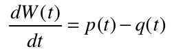
and
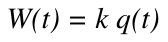
where W(t) is the volume of water stored in the catchment at time t, p(t) is rainfall, q(t) is the river flow at time t and k is a constant parameter with the dimension of time (if the parameter was not constant the model would not be linear).
The second equation above assumes a linear relationship between discharge and storage into the catchment. The properties of a linear function are described here. Actually, the relationship between storage in a real tank and bottom discharge is an energy conservation equation that is not linear; in fact, it is given by the well-known Torricelli's law. Therefore the linearity assumption is an approximation, which is equivalent to assuming that the superposition principle applies to runoff generation. Actually, such assumption does not hold in practice, as the catchment response induced by two subsequent rainfall events cannot be considered equivalent to the sum of the individual catchment responses to each single event. However, linearity is a convenient assumption to make the model simpler and analytical integration possible.
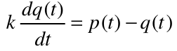
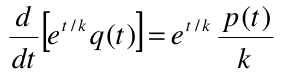
A nice feature of the linear reservoir is that the above equations can be integrated analytically, under simplifying assumption. In fact, by substituting the second equation into the first one gets:
Then, by multiplying both sides by et/k and dividing by k one gets:
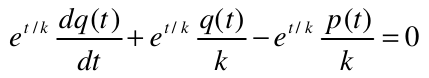
which can be written as:
By integrating between 0 and t one obtains:
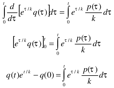
and, by assuming q(0)=0, one finally gets:
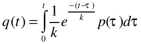
which can be easily integrated numerically by using the Euler method.
If one assumes p(t)=constant, an explicit expression is readily obtained for the river flow:
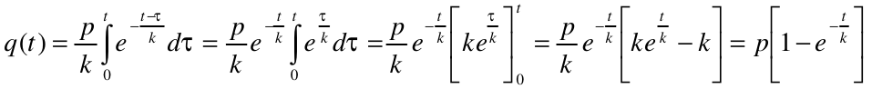
Figure 2 shows the progress of river flow with constant rainfall and Q(0)=0.
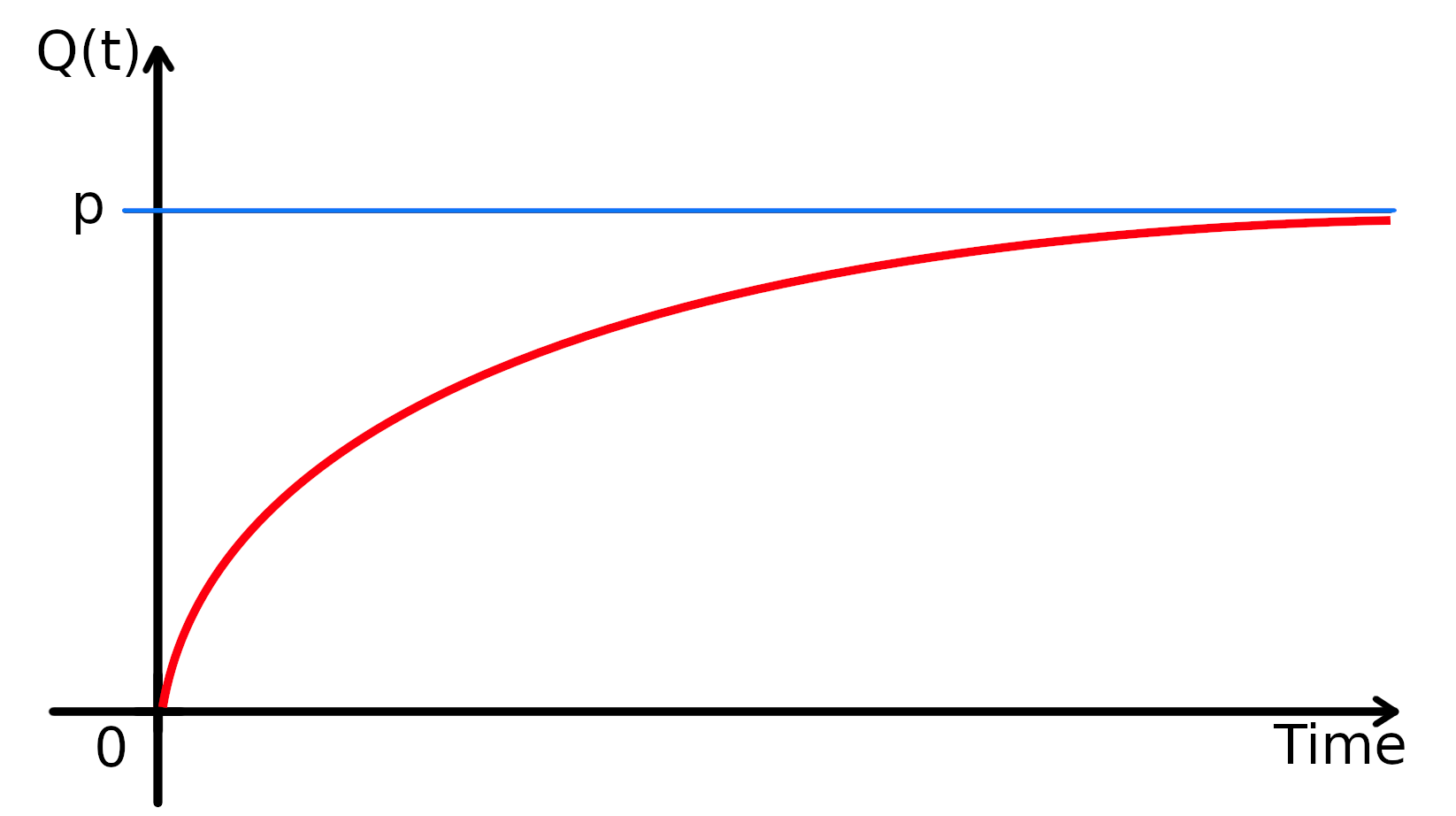
Figure 2. Output from the linear reservoir with constant rainfall and Q(0)=0.
The parameter k is usually calibrated by matching observed and simulated river flows. Its value significantly impacts the catchment response. A high k value implies a large storage into the catchment. Therefore, large values of k are appropriate for catchment with a significant storage capacity. Conversely, a low k value is appropriate for impervious basins. k is also related to the response time of the catchment. A low k implies a quick response, while slowly responding basins are characterised by a large k. In fact, k is related to the response time of the catchment. The linear reservoir is also described here.
Several variants of the linear reservoir modeling scheme can be introduced, for instance by adopting a non linear relationship between discharge and storage. Moreover, an upper limit can be fixed for the storage in the catchment, and additional discharges can be introduced, which can be activated for different levels of storage. All of the above modifications make the model non-linear so that an analytical integration is generally not possible. One should also take into account that increasing the number of parameters implies a corresponding increase of estimation variance and therefore simulation uncertainty. Furthermore, it is often observed that introducing additional discharges or thresholds may induce discontinuities in the hydrograph shape. The non-linear reservoir is described here.
 Figure 3. A non-linear reservoir (from Wikipedia)
The Hymod model is a flexible solution that is increasingly adopted for its capability of providing a good fit in several practical applications. It was originally proposed by Boyle (2000). It is based on the assumption that each point location i in the basin is characterised by a local value of soil water storage Ci, which varies from 0 in the impervious areas up to a maximum value Cmax in the most permeable location of the catchment. Ci is assumed to be randomly varying, so that for an assigned value C* of soil water storage a probability distribution is introduced that gives the probability that a randomly selected location j is characterised by Cj less then, or equal to, C*. Such probability may be interpreted as the fraction F(C*) of the catchment area where Cj≤C*. The above probability distribution is written as 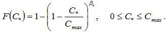 Here, βk is a parameter which quantifies the variability of the soil water storage over the catchment. One can easily verify by numerical simulation that βk=0 implies that the soil water storage is constant over the basin and equal to Cmax; βk=1 implies that the soil water storage is linearly varying from 0 to Cmax; βk→∞ implies that the soil water storage is tending to the null value over the whole catchment, which is therefore impervious.
Figures from 4 to 8 show the shape of the distribution function that is obtained for different βk values (note that βk is indicated with the symbol β in the graph titles).
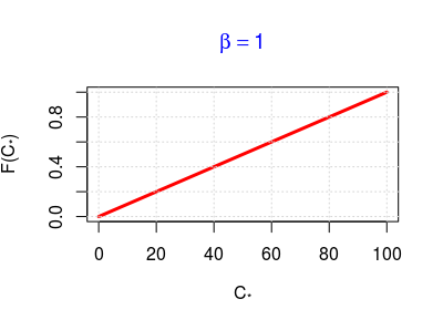
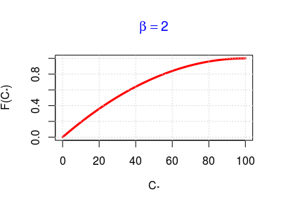
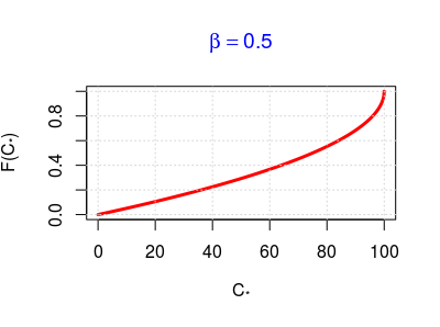
Figure 4, 5 and 6. Shape of the Hymod probability distribution for different values of βk.
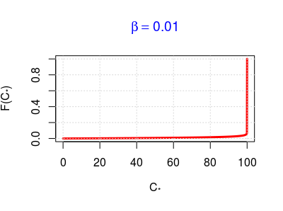
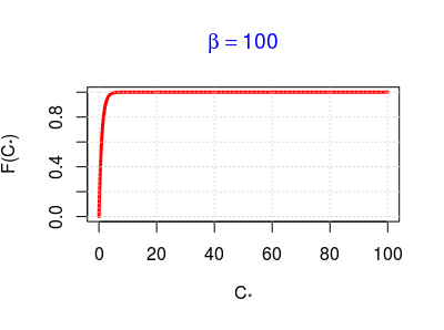
Figure 7 and 8. Shape of the Hymod probability distribution for extreme values of βk.
Numerical simulation to obtain the above figures can be carried out with the sample R script that follows (note the graphic instructions):
hymod=function(betak,cmax=100) { cstar=seq(0,cmax,0.1) Fcstar=1-(1-cstar/cmax)^betak # cat(titolo, fill=T) plot(cstar,Fcstar,type="l",ylim=c(0,1),xlab=expression("C"["*"]), ylab=expression("F(C"["*"]*")"), col="red",lwd=3,main=bquote(beta == .(betak)),col.main="blue") grid() }
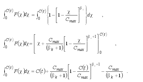
Let us assume that a storm event occurs over the basin and let us define with the symbol C(t) the time varying water depth stored in the unsaturated locations of the catchment. If we ignore any water losses, like evapotranspiration, C(t) is equal to the rainfall amount from the beginning of the event, which we will indicate with the symbol P(t). If one now substitutes C* with C(t) in the above probability distribution function, then the obtained relationship will describe the probability distribution of saturated area into catchment. Such distribution, now expressed in terms of C(t), is the one reported in Figure 9. It can be easily proved that the water volume stored in the catchment at time t is given by 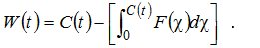
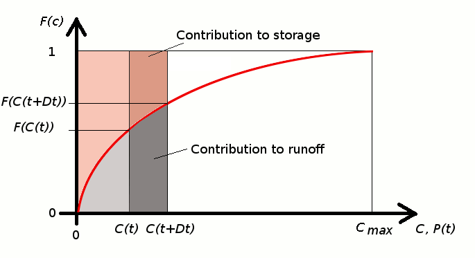
Figure 9. Distribution of soil water storage, surface runoff and stored volume in Hymod
In fact, the integral at the right hand side of the above equation is the area below the red line in Figure 9. Elementary increment of that area are given by the product of the rainfall at each time increment by the fraction F(c(t)) of saturated area at the same time, namely, the product of rainfall by saturated area, which is indeed the surface runoff. Conversely, the area above the curve gives the global storage into the catchment W(t), which can be interpreted as a weighted average value of C(t). The progress of surface runoff and water storage is depicted by the animated picture in Figure 10. Note that after saturation, the contribution of surface runoff is given by the product of the rainfall itself by 1, which is the fraction of saturated area, taking and keeping unit value when the catchment is saturated. After saturation, the storage in the catchment of course does not increase any more.

Figure 10. Progress of surface runoff and stored volume in Hymod
By computing the integral in the latter relationship, with the initial condition C(0) = 0, one obtains:
Therefore the water volume stored in the catchment is equal to
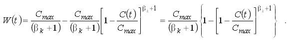
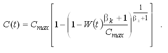
By inverting the above equation one gets
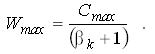
Note that one obtains an estimate of the upper value of the water volume that the catchment can store by imposing C(t)=Cmax, therefore obtaining
The above equations allow an easy application of the Hymod model through a numerical simulation, that is usually carried out by adopting a time step Dt that is equal to observational time step of rainfall and river flow. At a given time step t, one knows the value of C(t) which is equal to the cumulative rainfall depth from the beginning of the event at time t. Therefore, W(t) can be easily computed as well by using the above relationships. At the time t+1, C(t+1)=C(t)+P(t), where P is rainfall, under the condition that C(t+1)=Cmax if C(t)+P(t)>Cmax. Therefore, one can compute a first contribution to surface runoff through the relationship ER1(t)=max(C(t)+P(t)-Cmax,0).
Finally, one can compute a second contribution to the surface runoff which is given by the water volume that cannot be absorbed by the catchment because part of the catchment area got saturated in the last time step. Such second contribution is given by
ER2(t)=(C(t+1)-C(t))-(W(t+1)-W(t)).
By summing ER1+ER2 one obtains the total contribution to the surface runoff during the time step from t to t+1.
At this stage, one may evaluate the water losses given by evapotranspiration at the current time step, and subtract them from W(t+1). Such water losses are computed within Hymod through the relationship
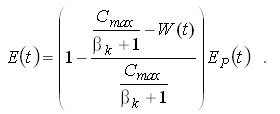
Here, Ep(t) is the potential evapotranspiration at time t. Then, the water storage at time t+1 is given by W(t+1)=W(t)-E(t).
One should note that the evapotranspiration is subtracted from the stored water volume after ER1 and ER2 are computed.
The total contribution ER(t)=ER1(t)+ER2(t) to the surface runoff is then divided into 2 components: αER(t) which represent the fast runoff and (1-α)ER(t) which is the slow runoff. αER(t) is propagated through a series of linear reservoirs with the same bottom discharge time constant kq, while (1-α)ER(t) is instead propagated through a single linear reservoir with parameter ks.
The computation moves forward through the sequence of time steps. Hymod counts 5 parameters, namely: Cmax, β, α, kq and ks. These parameters need to be calibrated by using observed data.
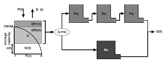
Figure 11. A schematic representation of the Hymod model
Groundwater models are computer models of groundwater flow systems. As for rainfall-runoff models, there are several different variants of groundwater models, but the physical principles are the same as for surface models: the conservation of mass and momentum. Groundwater models can be coupled with chemical and/or ecological models to describe water quality therefore allowing to design conservation and remediation strategies.
Groundwater models are based on the application of the groundwater flow equation. It can be derived by referring to a control volume where the properties of the medium are assumed to be constant, which in technical applications is the region of space occupied by an aquifer. Let us assume that:
- Fluid is incompressible;
- There are no sources of water mass in the control volume,
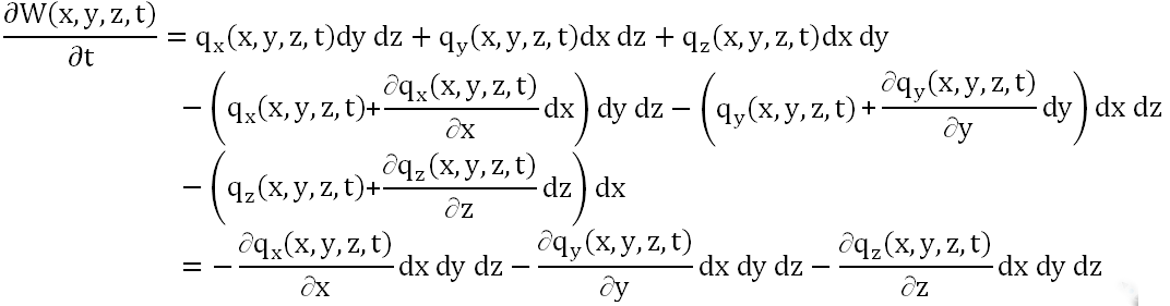
and let us denotes with W(x,y,z,t), Qin(x,y,z,t) and Qout(x,y,z,t) the water storage, total inflow into, and total outflow from, respectively, the elementary volume with coordinates x,y,z at time t (see Figure 12). Then, the continuity equation (see Figure 12) states that:

To estimate Qin(x,y,z,t), one may write:
- Volume per unit time into face x = qx(x,y,z,t)Ax = qx(x,y,z,t) dy dz;
- Volume per unit time into face y = qy(x,y,z,t)Ay = qy(x,y,z,t) dx dz;
- Volume per unit time into face z = qz(x,y,z,t)Az = qz(x,y,z,t) dx dy.
where qx(x,y,z,t), qy(x,y,z,t) and qz(x,y,z,t) are volumes per unit time and area of the control volume through the faces x, y and z, respectively.
Therefore the total inflow volume per unit time may be written as:
Qin(,y,z,t) = qx(x,y,z,t) dy dz + qy(x,y,z,t) dx dz + qz(x,y,z,t) dx dy .
The total outflow volume Qout(t) per unit time may be written as:
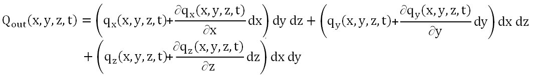 .
.
Therefore, one may write that:
 .
.
We now define Ss as the volumetric specific storage, which is often simply called specific storage: it is the volume of water that an aquifer releases from storage, per volume of aquifer, per unit decline in hydraulic head h(x,y,z,t) in the aquifer. It has the dimension of 1/length. Therefore, we can write that
 .
.
Thus, one obtains:

namely:

or, in compact form:
 .
.
This is known in other fields as the diffusion equation or heat equation. It is a parabolic partial differential equation.

Figure 12. A schematic representation of the control volume for a groundwater model
The above equation has both the flux q(x,y,z,t) and the head h(x,y,z,t) unknown. Therefore, it is necessary to couple the continuity equation with a second equation, which is the momentum equation that is derived from the Navier-Stokes equations. Under the assumption that the flow is slow and viscous, the momentum equation reduces to the Darcy's law, which is valid for laminar flow only (Reynolds number lower than 1) and reads as:
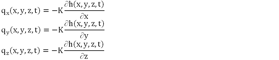
where K is hydraulic conductivity, which has the dimension of a velocity and is here assumed to be an isotropic property. By substituting in the above equation one obtains:

or

which is the desired groundwater flow equation. In steady-state conditions ∂ h(x,y,z,t)/∂ t = 0 and therefore the above equation reduces to Laplace equation which describes potential flow:
∇2h(x,y,z) = 0
which describes a potential flow. The latter is a flow field where the velocity field can be expressed as the gradient of a scalar function, namely, the velocity potential, which in the above case is the hydraulic head h(x,y,z).
To solve the groundwater flow equation for the sake of describing the hydraulic head, one needs to:
- specify the geometry of the control volume;
- specify the material properties (including hydraulic conductivity);
- specify the initial conditions;
- specify the boundary conditions;
- specify the method of solution.
Several groundwater models have been proposed by the literature which provide the above specifications by following different approaches and simplifications. In techincal applications several assumptions are ofter introduced like:
- steady-state flow;
- negligible vertical component of groundwater flow (Dupuit assumption), 2-dimensional model;
- negligible vertical and transversal component of groundwater flow, 1-dimensional model,
in order to simplify the problem.
Box 1: Volumetric specific storage and uncertainty
Volumetric specific storage, which represents the aquifer’s capacity to release or take in water when the head changes, is an important aquifer property required for water resources management. If the aquifer remains fully saturated, and therefore there is no reduction of saturated volume of the acquifer, the amount of water released is composed of two parts: the first is an expansion of water which occurs for decreasing head (head is equivalent to pressure into the acquifer); and the second is the compaction of the aquifer which again occurs for decreasing head.
Storativity of an aquifer is defined as the volume of water that is released by a vertical column of the aquifer of unit surface area per unit decline in hydraulic head. Note that surface area is lying over an horizontal plane under Dupuit's assumption of plane motion. For a confined aquifer the storativity is given by the product of specific storage and thickness. For an unconfined aquifer the storativity is given by the product of specific storage and initial saturated thickness of the aquifer.
For a confined aquifer, storativity results, as the specific storage, only from water and aquifer compressibilities and is typically very small. For an unconfined aquifer, the small effect of compressibilities is generally neglected (as the head is generally limited), and storativity is assumed to be equal to the specific yield, which is defined as the volume of water that will drain under the force of gravity from unit bulk volume of the aquifer. This is equal to the effective porosity (if one neglects the volume of water retained under gravity drainage by capillary forces).
Specific storage and storativity are essential in water resources management as they are crucial to quantify how much water an aquifer can deliver. It is usually defined with pumping tests and shows large variability even for similar aquifers. There is large uncertainty in the estimates. Estimation methods are still the subject of extended research.
Application of groundwater models is subjected to relevant uncertainty. Besides the usual approximation affecting environmental models, when dealing with groundwater one needs to face uncertainty originated by the limited knowledge of the geometry of the control volume and the physical and hydraulic properties of the porous media. Geological prospections and field measurements are needed in order to parametrize models and define initial and boundary conditions. Notwithstanding the presence of uncertainty, models deliver useful information that may allow one to integrate the assessment provided by inductive methods. However, uncertainty needs to be communicated to end users and policy makers, through a quantitative assessment.
Uncertainty may be quantitatively estimated by applying the theory of probability. Usual approaches are based on including an error term to model performances, which may be a multiplicative or additive factors. The error can be defined in probabilist terms, through model validation, which is essentially based on comparing model performances with observed data. Model calibration and validation is described here.
Another approach to quantify uncertainty is to run several model simulation for different geometric configuration of the control volume, different initial and boundary conditions and different parameters, therefore obtaining a range for the model output, which allows to define a range for the desired design variables.
Uncertainty assessment for hydrological models is still an active research field. Applications in the professional practice are still rare.
Boyle, D. P. (2000), Multicriteria calibration of hydrological models, Ph.D. dissertation, Dep. of Hydrol. and Water Resour., Univ. of Ariz., Tucson.
Download the powerpoint presentation of this lecture
Last modified on March 15, 2021
- 376 viste