1. Premise

Assessment of climate change and climate change impact is a key step for the design of climate change adaptation actions. Climate change impact assessments aims to characterize climate change and quantitatively estimate the risks or impacts of environmental change on people, communities, economic activities, infrastructure, ecosystems, valued natural resources. It also entails estimation of project risk.

While there are several guidelines suggesting concepts for climate change impact assessment, like for instance the EU Climate change policy suggesting the target of carbon neutrality by 2050, the quantitative estimation of climate induced risks under change depends on the local context and the vulnerability of local environment and communities. Traditional engineering methods assuming stationarity need to be revised and integrated with a technical assessment of the uncertainties induced by climatic transition.

To elaborate aquantitative assessment of climate change impact one posibility is to refer to risk based design:

\( R=PVE\)

where \(P\) is hazard, \(V\) is vulnerability and \(E\) is exposure (see here for more details). In particular, climate change affects hazard \(P\) which is usually estimated through probability theory. The challenge is to estimate hazard in future conditions which of course are not known at the moment, while we know that traditional probabilistic methods may be inadequate (may be, not for sure). We will denote future and unknown hazard conditions with the simbol \(\hat P\). 

Climate change impact assessment - and therefore future hazard \(\hat P\) - may be carried out through deductive or inductive reasoning. Science itself is an interplay between deductive and inductive reasoning.  Inductive reasoning means that a general principle is derived from a body of observations. Deductive reasoning is the process of drawing conclusions as logical elaboration from their premises.

Both inductive and deductive reasoning may be used to carry out:

• Quantitative estimation of past climate change;
• Future climate change projections along with uncertainties;
• Assessment of climate change impact.

2. Inductive quantitative estimation of climate change: Historical data analysis

Historical data analysis is a frequently used approach to assess climate change. It has been recently criticized because the representativity of past data to assess changes in environmental variables has been widely questioned, for the presence of errors and gaps in observations and the reduced spatial density of monitoring stations. In several cases questions arise on the homogeneity of data, for example, about whether the series is equally reliable throughout its length.

In hydrology and water resources management past data analysis is usually preferred for the applied character of the related assessments. When project variables are to be determined in practice, data analysis is frequently considered the most reliable approach, allowing a convincing estimation of uncertainty.

Several approaches can be applied to assess change, and therefore human impact, by analysing historical environmental data. We will focus on trend analysis, which can applied to assess the tendency of any observed time series. We will also discuss run theory, that is frequently used to assess drought, and estimation of long term persistence, which is related to the tendency of a process to exhibit long term cycles. Several additional techniques and examples for historical data analysis could be discussed. Besides examples and details, it is important to understand the concept underlying historical assessment of climate change: through the past evidence of climate change, as it appears from observations, we try to quantify the transitional behaviour of climate and its future evolution.

2.1. Trend Analysis

The most used approach is trend analysis of a historical time series. If the trend can be assumed to be linear, trend analysis can be undertaken through regression analysis, as described in trend estimation. If the trends have other shapes than linear, trend testing can be done by non-linear methods.

Linear trend estimation is essentially based on fitting a linear straight line interpolating the data. A linear function f(x) must satisfy two conditions:

• \(f(a + x) = f(a) + f(x)\)
• \(f(ax) = a f(x)\).

Therefore, a given time series y(t) is assumed to be decomposed in a straight line plus a noise:

\(y(t) = a + bt + \epsilon(t)\)

where \(a\) and \(b\) are the intercept and slope of the trend line, respectively, and \(\epsilon(t)\) is a randomly distributed residual whose statistical properties are assumed not to change in time. If the slope b is significantly positive or negative, then a trend in the data exists which provides an indication of the related change. This approach is indicated for the estimation of changes that are gradually occurring in time, while it is not representative of sudden changes like river diversions, river damming or the perturbation given by other infrastructures.

To estimate \(a\) and \(b\) and the statistical behaviors of \(\epsilon(t)\), which can be considered as parameter of the above linear model, the least squares approach is usually applied.This method minimizes the sum of the squared values of \(\epsilon(t)\), as computed by the difference between the y(t) values and the available and corresponding observations:

\(\mbox{min} \sum_{t=1}^N(y(t) - a - bt)^2\)

where \(y(t)\) is the observation and \(N\) is the number of observed data. By using proper inference methods a confidence band can be computed for the value of the slope. In statistics, confidence bands or confidence intervals potentially include the unobservable true parameter of interest. How frequently the estimated confidence band contains the true parameter if the experiment is repeated on different time series is called the confidence level.

More generally, given the availability of a hypothesis testing procedure that can test the null hypothesis \(b = 0\) against the alternative that \(b \neq 0\), then a confidence interval with confidence level \(\gamma = 1 − \alpha\) can be defined as the interval around 0 containing any \(b\) value for which the corresponding null hypothesis \(b = 0\) is not rejected with probability \(1 − \alpha\). According to the above formulation, \(\alpha\) is called significance level.

Computation of the confidence interval is affected by the assumptions on \(\epsilon(t)\) and in particular the assumptions related to its probability distribution. Usually the residuals are assumed to follow a normal distribution and to be uncorrelated. These assumptions heavily impact the estimation of the confidence interval. In particular, the presence of correlation widens the width of the confidence interval significantly. Therefore, the question often arises on the possible presence of correlation in environmental variables, and in particular the present of correlation extended over long time ranges, which corresponds to the presence of long term cycles. If the considered time series is affected by such long term periodicities, then distinguishing between a linear trend and a long term cycle may be difficult. For instance, characterising the current trend that is observed in the global temperature is challenging if one accepts the idea that the climate system may be affected by such long term cycles.

An idea of the variability of environmental data and related tendencies and cycles may be given by Figure 1 and Figure 2, which display the progress of a trend line estimated in a moving window starting from 1920 and encompassing 50 observations of annual maxima (Figure 1) and annual minima (Figure 2) of the Po River daily flows at Pontelagoscuro. The considered time series is extended from 1920 to 2009 and therefore provides the opportunity of testing how the slope of the regression line changed along the observation period. Even if 50 years is a long period, which is usually considered extended enough to allow a reliable trend estimation, one can see that the slope of the regression line is continuously changing, therefore proving that natural fluctuations lead to considerable changes in the dynamics of the river flow which cannot be easily interpreted through a linear trend.

Figure 1. Regression line estimated along a moving window encompassing 50 years of annual maxima of the Po River at Pontelagoscuro. Increasing and decreasing slopes are depicted in red and blue, respectively.

Figure 2. Regression line estimated along a moving window encompassing 50 years of annual minima of the Po River at Pontelagoscuro. Increasing and decreasing slopes are depicted in blue and red, respectively.

Trend estimation is also used for elaborating future climatic projections, by projecting the estimated trend along the next years. One needs to be fully aware that uncertainty of extrapolations is different - likely higher - than uncertainty in interpolation.

2.2. Run theory

Run theory if frequently applied to assess the severity of droughts, in particular with respect to the long ones (Yevjevich, 1967). For the sake of providing an example, we will discuss run theory applied to annual rainfall to characterise drought events in terms of drought frequency, duration, severity and intensity.

Run theory has been applied in several areas worldwide (Ho et al., 2021; Wu et al., 2020; Mishra et al., 2009). In detail, the long term mean rainfall \(RLT\) is adopted as the threshold to identify positive or negative runs (see Figure 3). If rainfall in a given year is lower than an assigned threshold \(T_{lower} < RLT\) a negative run is started which ends in the year when the rainfall is higher than \(RLT\) . If the interval between two negative runs is only one year and rainfall in that year is less than a selected threshold \(T_{upper} > RLT\) , then these two runs are combined into one drought. Finally, only runs which have a duration of no less than \(n\) years are determined as multiyear drought events. To give an example, the thresholds \(T_{upper}\) and \(T_{lower}\) may be defined as 20% more and 10% less than \(RLT\) , respectively, and one can assume \(n=3\). Once a multiyear drought has been identified, drought duration is the time span between the start and the end of the event, and drought severity is computed as the cumulative rainfall deficit with respect to \(RLT\) during drought duration divided by the mean rainfall, and drought intensity is computed as the ratio between drought severity and duration. We also estimate the maximum deficit of the drought event, namely, the largest difference between annual rainfall and \(RLT\) during the event. Finally,drought frequency is computed as the ratio between the number of drought events that have been identified and the length of the observation period.

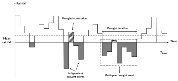
Figure 3: Run theory

2.3. Estimation of long term persistence

Long-range dependence (LRD), also called long memory or long-range persistence, is a behaviour that may be exhibited by time series. It relates to the rate of decay of statistical dependence (sometimes called "memory") of two points located progressively apart in time. A process is considered to exhibit long-range dependence if the above dependence decays more slowly than usual. With "usual" here we mean processes whose "memory" decays rapidly.

A way of characterizing long- and short-range dependence is by computing the variance of the mean value of consecutive values, which is expected to decrease for increasing number of observations. For short-range dependence, the variance declines proportionally to the inverse of the number of terms. In the presence of LRD, the variance of the mean value decreases slower (which means that estimation of the mean value is more uncertain), for the presence of long term cycles which increase variability. In particular, in the presence of LRD the decline of the variance of the mean is described by a power function:

\(\mbox{Var}(\hat X_N)\sim cN^{2H-2}\)

where \(c>0\) and \(\hat X_N\) is sample mean. If \(H=0.5\) we are in the presence of short term dependence, while for \(H>0.5\) (and less than 1 for reasons which we do not discuss here) we have LRD. \(H\) is called the "Hurst exponent": it is a measure of the intensity of LRD.

We do not discuss LRD further but want to enphasise here that LRD may be the explanation for events like:

• Millenium drought in Australia;
• Drought in California;
• Drought in South Africa.

For an interesting short history of how LRD was discovered and how the Hurst exponent was defined see this presentation illustrating a game changer discovery in science.

Deductive assessment of climate change and its impact may be carried out by applying mathematical models which simulate the considered Earth system processes. There are typically physical models, which may however involve chemical, biogeochemical and other components. In their physical components, these models frequently describe the storage and flow of physical matters, through conservation equations. In particular, conservation of mass, energy and momentum are frequently applied.

We will discuss here the simple example of climate models which can be used to quantify both past and future climate change. To estimate future projections for other specific variables, transformation models may be used to propagate the change in climate thus estimating change for impact-specific statistics. For instance, energy models can be used to estimate how climate change impacts the production of energy through, e.g., wind farms.

To provide a more practical and technical example, we discuss here below to rainfall-runoff models which are frequently used to assess the impact of climate change on water resources and water related risks.

3.1. Climate modelling and bias correction

Past and future predictions by climate models can be easily retrieved from several public repositories. One interesting example is the Copernicus Climate Data Store which provides data for Europe at very fine spatial and temporal resolution. For instance, one can find there reconstructions of past and future climate in Bologna from more than 10 global climate models.

Past reconstructions are useful because one can check the reliability and uncertainty of models to reproduce the past climate. Basing on model errors uncertainty of future predictions may be estimated. Furthermore, model performances in the reproduction of observed data may be used to make corrections to model predictions.

In fact, climate models have systematic errors (biases) in their output. For example climate models often have too many rainy days and tend to underestimate rainfall extremes. There can be errors in the timing of the extremes or the average of seasonal temperatures, which can be consistently too high or too low.

To correct biases in climate models, a range correction methods have been developed. These methods can be applied only when observed historical data are available. In fact, the quality of the observational datasets determines the quality of the bias correction.

The simplest approach to bias correction is the Delta change method. Accordingly, models are used to predict change rater than the future value of a given variable. For instance, if the climate model predicts 3°C higher temperatures for a given date in the future, then this rate of change in time is added to all historic observations to construct a new scenario for the future climate. The percentage change is usually calculated and used to correct bias.

It is important to take into account that bias correction only adjusts specific statistics, like the average value, while errors may remain in the reproduction of other statistics, like for instance variance. To correct the bias for ungauged locations extrapolation methods can be used.

3.2. Rainfall-runoff modelling

Rainfall-Runoff modeling is one of the most classical applications of hydrology. It has the purpose of simulating a river flow hydrograph in a given cross river section induced by an observed or a hypothetical rainfall forcing. Rainfall-runoff models may include other input variables, like temperature, information on the catchment or others. Within the context of this subject, we are studying rainfall-runoff models with the purpose of producing simulation of long term hydrographs.

Rainfall-runoff models describe a portion of the water cycle (see Figure 1) and therefore the movement of a fluid - water - and therefore they are explicitly or implicitly based on the laws of physics, and in particular on the principles of conservation of mass, conservation of energy and conservation of momentum. Such conservation laws apply to a control volume which includes the catchment and its underground where water flow takes place. The catchment is defined as the portion of land whose runoff uniquely contributes to the river flow at its closure river cross section.

Depending on their complexity, rainfall-runoff models can also simulate the dynamics of water quality, ecosystems, and other dynamical systems related to water, therefore embedding laws of chemistry, ecology, social sciences and so forth.

Models are built by constitutive equations, namely, mathematical formulations of the above laws, whose number depends on the number of variables to be simulated. The latter are the output variables, and the state variables, which one may need to introduce to describe the state of the system. Constitutive equations may include parameters: they are numeric factors in the model equations that can assume different values therefore making the model flexible. In order to apply the model, parameters needs to be estimated (or calibrated, or optimized, and we say that the model is calibrated, parameterized, optimized). Parameters usually assume fixed value, but in some models they may depend on time, or the state of the system.

Figure 4. The hydrologic cycle (from Wikipedia)

Rainfall-runoff models can be classified within several different categories. They can distinguished between event-based and continuous-simulation models, black-box versus conceptual versus process based (or physically based) models, lumped versus distributed models, and several others. It is important to note that the above classifications are not rigid - sometimes a model cannot be unequivocally assigned to one category. We will treat rainfall-runoff models by taking into consideration models of increasing complexity.

The Rational Formula delivers an estimate of the river flow \(Q\) [L³/T] for a catchment with area \(A\) [L²], depending on a forcing given by rainfall intensity \(i\) [L/T] and the runoff coefficient \(C\) [-]. The rational formula can be considered the first rainfall-runoff model proposed. It was developed by the American scientist Kuichling in 1889, who elaborated concepts that were previously proposed by the Irish engineer Thomas Mulvaney in 1851. Although very simple, the Rational Formula is extremely useful in hydrology to increase the physical basis when estimating peak flow and to get baseline estimates. Being focused on the estimation of peak river flow, the rational formula is not generally used to assess water resources availability. The Rational Formula reads as:

\(Q = C i A,\)

it is dimensionally homogeneous and therefore one should measure rainfall in m/s and the catchment area in \(m^2\) to obtain an estimate of the river flow in \(m^3/s\).

A relevant question is related to the estimation of the rainfall intensity \(i\) to be plugged into the Rational Formula. It is intuitive that an extreme rainfall estimate should be used, which is related to its return period and the duration of the event. The return period is defined as the average time lapse between two consecutive events with rainfall intensity reaching or exceeding a given threshold. In fact, an empirical relationship, the depth-duration-frequency curve, is typically used to estimate extreme rainfall depending on duration and return period.

When applying the Rational Formula, one usually assumes that the return period of rainfall and the consequent river flows are the same. This is assumption is clearly not reliable, but nevertheless is a convenient working hypothesis. Further explicit and implicit assumptions of the Rational Formula are not discussed here. As for the duration of the rainfall event, it can be proved, under certain assumptions, that the rainfall duration that causes the most severe response by the catchment, in terms of peak flow, is equivalent to the time of concentration of the catchment. The time of concentration is defined as the time needed for water to flow from the most remote point in a watershed to the watershed outlet.It is important to note that the mean areal rainfall intensity over the catchment should be plugged into the rational formula. Therefore, for large catchments (above 10 \( km^2 \)) one should estimate \( i \) by referring to a central location in the catchment and an areal reduction factor should be applied.

Let us note that the rational formula is implicitly based on the principle of mass conservation. There is also the implicit use of the principle of conservation of energy in the estimation of the time of concentration. In fact, even if such time is estimated empirically, the mass transfer to the catchment outlet is actually governed by transformation and conservation of energy.

3.2.2. The linear reservoir

The linear reservoir is one of the most used rainfall-runoff models, together with the time area method (see also this link)which we will not discuss here. The linear reservoir model assimilates the catchment to a reservoir, for which the conservation of mass applies. The reservoir is fed by rainfall, and releases the river flow through a bottom discharge, for which a linear dependence applies between the river flow and the volume of water stored in the reservoir, while other losses - including evapotranspiration - are neglected. Therefore, the model is constituted by the following relationships:

\(\frac{dW(t)}{dt}=p(t)-q(t)\)

and

\(W(t)=kq(t)\)

where \(W(t)\) is the volume of water stored in the catchment at time \(t\), \(p(t)\) is rainfall volume per unit time over the catchment, \(q(t)\) is the river flow at time \(t\) and \(k\) is a constant parameter with the dimension of time (if the parameter was not constant the model would not be linear).

The second equation above assumes a linear relationship between discharge and storage into the catchment. The properties of a linear function are described here. Actually, the relationship between storage in a real tank and bottom discharge is an energy conservation equation that is not linear; in fact, it is given by the well-known Torricelli's law. Therefore the linearity assumption is an approximation, which is equivalent to assuming that the superposition principle applies to runoff generation. Actually, such assumption does not hold in practice, as the catchment response induced by two subsequent rainfall events cannot be considered equivalent to the sum of the individual catchment responses to each single event. However, linearity is a convenient assumption to make the model simpler and analytical integration possible.

A nice feature of the linear reservoir is that the above equations can be integrated analytically, under simplifying assumption. In fact, by substituting the second equation into the first one gets:

\(k\frac{dq(t)}{dt}=p(t)-q(t)\)

Then, by multiplying both sides by e^t/k and dividing by k one gets:

\(e^{t/k}\frac{dq(t)}{dt}+e^{t/k}\frac{q(t)}{k}-e^{t/k}\frac{p(t)}{k}=0\)

which can be written as:

\(\frac{d}{dt}\left[e^{t/k}q(t)\right]=e^{t/k}\frac{p(t)}{k}\)

By integrating between 0 and t one obtains:

\(\int_0^t \frac{d}{dt}\left[e^{\tau/k}q(\tau)\right]d\tau=\int_0^t e^{\tau/k}\frac{p(\tau)}{k} d\tau\)

and then

\(\left[e^{\tau/k}q(\tau)\right]^t_0 =\int_0^t e^{\tau/k}\frac{p(\tau)}{k} d\tau,\)

\(e^{t/k}q(t)-q(0)=\int_0^t e^{\tau/k}\frac{p(\tau)}{k} d\tau,\)

and, by assuming \(q(0)=0\) one gets:

\(q(t)=\int_0^t \frac{e^{\tau/k}}{e^{t/k}}\frac{p(\tau)}{k} d\tau,\)

and, finally,

\(q(t)=\int_0^t \frac{1}{k}e^{\frac{-(t-\tau)}{k}}p(\tau)d\tau\)

which can be easily integrated numerically by using the Euler method.

If one assumes p(t)=constant, an explicit expression is readily obtained for the river flow:

\(q(t)=\frac{p}{k}\int_0^t e^{\frac{-(t-\tau)}{k}}d\tau\)

\(q(t)=\frac{p}{k}e^{-\frac{t}{k}}\int_0^t e^{\frac{\tau}{k}}d\tau\)

\(q(t)=\frac{p}{k}e^{-\frac{t}{k}}\left[ke^{\frac{\tau}{k}}\right]_0^t\)

\(q(t)=\frac{p}{k}e^{-\frac{t}{k}}\left[ke^{\frac{t)}{k}}-k\right]\)

\(q(t)=p\left[1-e^{-\frac{t}{k}}\right].\)

Figure 2 shows the progress of river flow with constant rainfall and Q(0)=0.

Figure 5. Output from the linear reservoir with constant rainfall and Q(0)=0.

The parameter k is usually calibrated by matching observed and simulated river flows. Its value significantly impacts the catchment response. A high k value implies a large storage into the catchment. Therefore, large values of k are appropriate for catchment with a significant storage capacity. Conversely, a low k value is appropriate for impervious basins. k is also related to the response time of the catchment. A low k implies a quick response, while slowly responding basins are characterised by a large k. In fact, k is related to the response time of the catchment. The linear reservoir is also described here.

Several variants of the linear reservoir modeling scheme can be introduced, for instance by adopting a non linear relationship between discharge and storage. Moreover, an upper limit can be fixed for the storage in the catchment, and additional discharges can be introduced, which can be activated for different levels of storage. All of the above modifications make the model non-linear so that an analytical integration is generally not possible. One should also take into account that increasing the number of parameters implies a corresponding increase of estimation variance and therefore simulation uncertainty. Furthermore, it is often observed that introducing additional discharges or thresholds may induce discontinuities in the hydrograph shape. The non-linear reservoir is described here.

Figure 6. A non-linear reservoir (from Wikipedia)

3. Estimation of future forcing

Both historical analysis and modelling can be used to estimate future design events under climate change. In some cases - for instance where historical data are lacking - only the modelling approach will be possible. In other cases bot approaches may be applied.

Note that it is not possible to predetermine which approach will lead to the more conservative estimate. The results depend on the local context and uncertainty. Integration of methods and comparison of the results, therefore using any possible source of information, is the most desired approach.

References

Yevjevich, V. (1967) An Objective Approach to Definitions and Investigations to Continental Hydrologic Droughts. Colorado State University, Fort Collins, Colorado.

Last updated on March 26, 2023