
The "spheres" of the Earth system and their connections
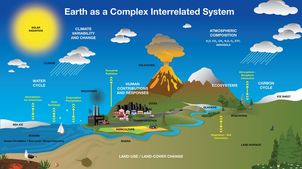
The Earth system identifies the unified whole resulting from the aggregation of interrelated entities that are relevant to the dynamic evolution of the planet Earth and its atmosphere. The Earth system is closed, meaning that only energy can flow in and out, with the only exception of masses that can enter from space, like meteorites. Entities include the dynamic processes that connect the different parts of the system itself (Figure 1).
The modern holistic view of the Earth system as a unified whole, rather than the aggregation off distinct parts and processes, emphasizes the importance of the intimate relations among entities, which include the feedbacks. Criticism to the holistic view points out that these intimate relations can only be modelled through complex mathematical representation which may be difficult to parametrise.
The traditional reductionist view represents the Earth system as an aggregation of domains, called "spheres". Although outdated, this view is useful to understand the role of each entity. Spheres that are traditionally considered are:
- Atmosphere;
- Geosphere;
- Biosphere;
- Hydrosphere.
An interesting presentation of the above spheres and their connection is given in "The Earth System" from Geoscience Videos. Other spheres are often considered, like:
- Cryosphere (snow and ice);
- Lithosphere (land);
- Pedosphere (soil);
- Technosphere (humans).
It is interesting to focus on the links between spheres, in order to understand how they are connected and how they mutually react to changes. These links ensure the connection between spheres through flows of energy and matters. There are several links that can be considered within a reductionist view depending on the scientific perspective and interests.
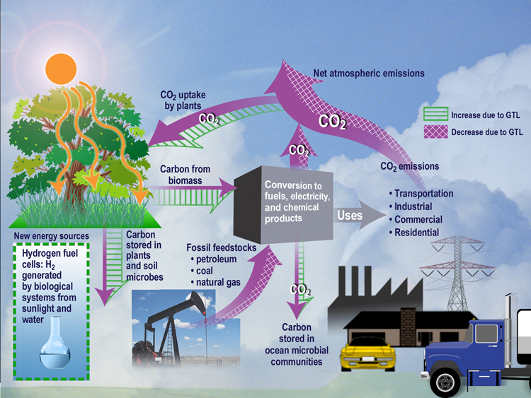
One possibility is to look at the carbon cycle as the agent linking the spheres. The carbon cycle describes the process in which carbon is exchanged from the atmosphere to the Earth (see this video from NOAA). The carbon cycle is a closed system, where only energy can enter and leave, while carbon cannot. The carbon cycle is fueled by energy from the Sun. Understanding perturbations of the carbon cycle - including the human induced ones - is instrumental to improve the assessment of climate change and its impacts (Figure 2).
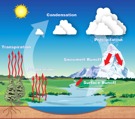
Another perspective to look at the links between spheres within a reductionist view is offered by the water cycle, that describes how water is exchanged through the different spheres through water flow, evaporation by living organisms and matters, precipitation and other phenomena (see Figure 3). Like the carbon cycle, the water cycle is fueled by energy from the Sun and impacted by humans and other living entities. This video by Nasa provides an introductory overview to the water cycle. See also this video by ESA.
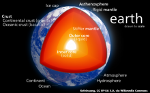
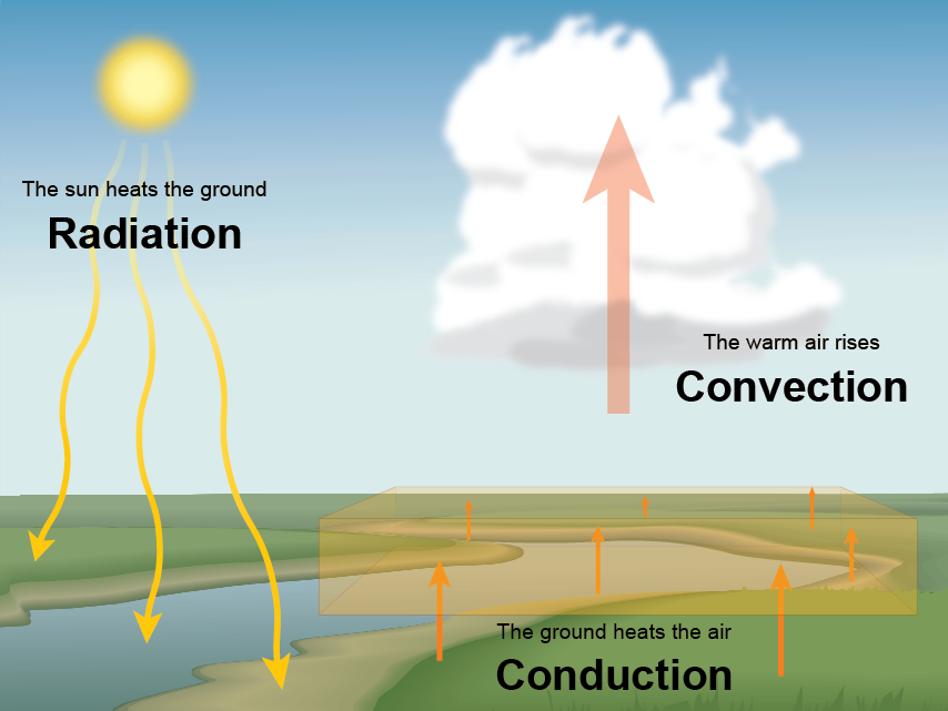
Another perspective on the links among spheres is offered by energy exchanges. If we focus on Earth and atmosphere, it is interesting to look at the balance between incoming energy from the Sun and outgoing energy from the Earth. Heat energy comes from the Sun through radiation, and is exchanged in the Earth system through conduction and convection (Figure 4). When it reaches the Earth, some energy from the sun is reflected back to space by clouds, some is absorbed by the atmosphere, and some is absorbed at the Earth's surface.
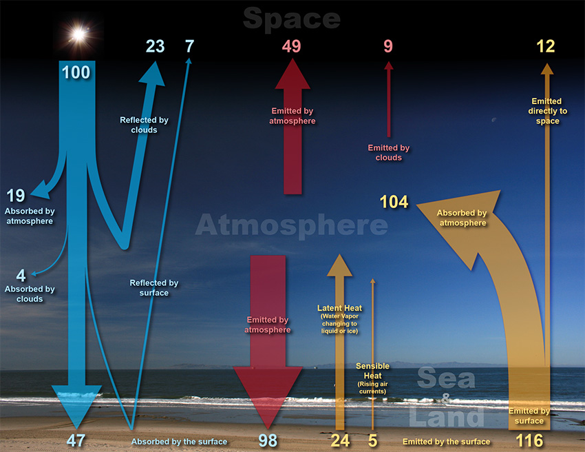
A quantitative look at energy balance in the Earth system is offered by Figure 5. It is interesting to look at the orders of magnitude, that help one to realise what are the most important processes.
All of the above cycles are closely interconnected. Carbon exchanges are related to water exchanges, while both of them depend on energy exchanges, as we pointed out above. The presence of multiple and multifaceted links is one of the reasons of the Earth system's complexity, which makes the holistic view difficult to translate into mathematical schemes. On the one hand, describing all of the above links is necessary for gaining an understanding of the system. On the other hand, a complete mathematical description would be difficult to manage, for the presence of uncertainty and chaotic behaviors.
Above all, we still have a limited knowledge of the links themselves, and therefore we cannot formulate a fully deterministic description. To provide an example of the unknowns, it is interesting to look at this blog post hosted by the European Geosciences Union (it is the fifth post in a series of 5; links to the previous ones are provided therein). One may also look at the interesting initiative of the International Association of Hydrological Sciences, the 23 unsolved problems in hydrology.
Dynamics of the Earth system
The many interrelations and feedbacks among the several subsystems of the Earth system are governed by complex dynamics, that are characterised by strong nonlinearities and tipping points. The resulting system is highly sensitive to initial conditions and certain perturbations. While some imposed changes would not alter the state of the system - even if they are relevant - some other tiny changes may lead to a significant perturbation of the system which may degenerate to significantly different condition through an irreversible process.
Box: Non-linearity
In mathematical terms, a linear function \(f(x)\) is the one that satisfies both of the following conditions:
- Additivity or superposition principle: \(f(x+y)=f(x)+f(y)\);
- Homogeneity: \(f(\alpha x)=\alpha f(x)\).
Additivity implies homogeneity for any rational \(\alpha\), and, for continuous functions, for any real \(\alpha\). For a complex \(\alpha\), homogeneity does not follow from additivity. Plotting a linear relationship in a graph originates straight line, while a nonlinear relationship creates a curve, which may be characterised by strong gradients in the dependent variables. In fact, in a nonlinear system the change of the output is not proportional to the change of the input. It follows that a nonlinear system may be subjected to significant changes of the output after tiny changes of the input. Thus, it is more difficult to predict as errors in the input variables may originate large uncertainties in the output.
Box: Tipping points
A tipping point for a given system (like the climate systems) is a state of the system such that a tiny change of the state itself leads to a new equilibrium state. The tipping point may be reversible or not. Tipping points may be induced by positive (self-reinforcing) feedbacks. Components of the Earth system that may pass a tipping point have been referred to as tipping elements. (see Figure 3). Tipping elements are found in the Greenland and Antarctic ice sheets, possibly causing tens of meters of sea level rise. The IPCC states that the precise levels of climate change sufficient to trigger a tipping point remain uncertain, but that the risk associated with crossing multiple tipping points increases with rising temperature.
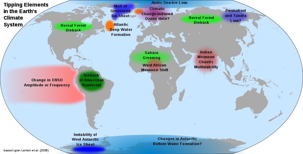
Figure 3. Tipping elements in the Earth's climate system, based upon Lenton et al. (2008). By CodeOne (blank map), DeWikiMan (additional elements), https://en.wikipedia.org/wiki/File:Climate-tipping-points-en.svg.
Figure 4 depicts examples of social tipping points which can trigger abrupt changes in the social system. It also depicts possible interventions for reaching the target of carbon neutrality.
The mechanisms leading to trespassing tipping points are not yet fully understood and therefore they may be not reliably reproduced by climate models. This may cause climate simulations to underestimate the risk of extreme events.
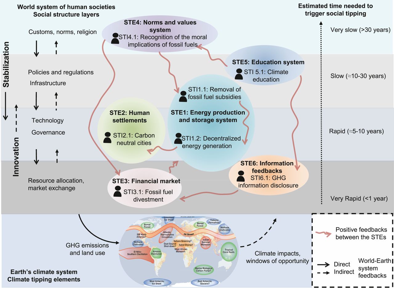
Figure 4. Social tipping elements and associated social tipping interventions with the potential to drive rapid decarbonization in the World–Earth system. By Otto et al., 2020. CC BY 4.0, https://commons.wikimedia.org/w/index.php?curid=87320451.
The presence of complexity and chaotic behaviours implies the presence of uncertainty, this implying the problem of how to represent it. Beware that the presence of uncertainty means the impossibility to obtain a precise prediction, but a prediction is still possible although affected by uncertainty. The classic approach to deal with uncertainty is through probability theory and therefore prediction - in the presence of uncertainty- is possible only in probabilistic terms. Other approaches can be adopted to represent uncertainty, like fuzzy logic or possibility theory. They all end up with an imprecise prediction.
The presence of uncertainty thus implies that the predictive models are formulated in probabilistic terms. Beware that a probabilistic model may contain a deterministic process based component, which is tasked of exploiting the information that we have on the considered system.
Mathematical models of the Earth system
To cope with the impact of climate change and to design climate change adaptation actions we need to predict a future design event under the impact of climate change. To obtain a quantitative estimate the event is associated to a number that is called the design load or project design variable. For the purpose of project design, we also need to provide an uncertainty assessment for such variable.
Predictions for the Earth system are obtained by applying mathematical models, that may have different structure depending the information they use and the underlying assumptions. Understanding and describing the internal dynamics and the many links of the spheres of the Earth systems is essential to make prediction of the future evolution of the environment and climate. Many different models can be used depending on how essential elements of the Earth system are interpreted and described.
Models can be classified within several different categories. They can distinguished between event-based and continuous-simulation models, black-box versus conceptual versus process based (or physically based) models, lumped versus distributed models, and several others. It is important to note that the above classifications are not rigid - sometimes a model cannot be unequivocally assigned to one category.
Process-based (or physically-based) models attempt to describe the internal processes of the spheres and the links between spheres basing on the law of physics and in particular conservation equations. These are often expressed in differential forms as they typically describe changes in variables that occur within an infinitesimal time and/or spatial step. The number of equations depends on the number of output variables from models and the number of associated state variables. Differential equations need to be integrated if one wishes to obtain an explicit equation that provides the desired output variables. Integration may be obtained by analytical or - more often - numerical integration depending on initial and boundary conditions.
An alternative to process-based models is given by the so-called empirical models that provide an analytical interpretation of evidence rather than an interpretation of the underlying system. Empirical models may be obtained by simplifying process-based ones and may implicitly or explicitly incorporate process-based principles. For instance, the linear reservoir model that is used to model parts of the water cycle is an empirical solution that is composed by a process-based mass balance equation and an empirical form of conservation of energy.
Both process-based and empirical models may have stochastic or deterministic structure.
Box: deterministic vs stochastic model
A deterministic model provides an outcome that is precisely determined through a known relationship between states and events. For a given input, state and conditions the model always reproduces the same output with no uncertainty.
A stochastic model derives all possible outcomes from a given process by using random information like input variables and initial and boundary conditions. The outcomes are presented through their probability distribution that gives an estimate of the expected frequency of each single output.
While the deterministic approach may look simpler than a stochastic one, actually the stochastic model is nothing else than an ensemble - obtained in rigorously codified way - of deterministic simulations. While the deterministic approach associates to one input only one output (one-to-one association) with no uncertainty, the stochastic models associates many inputs to many outputs therefore incorporating uncertainty assessment (see figure 6).
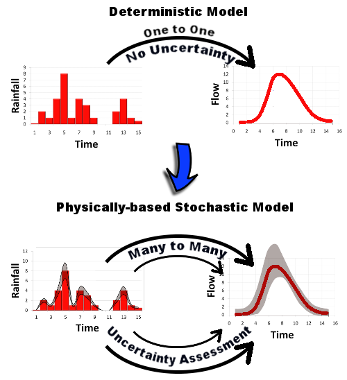
Figure 3. Determinsitic versus stochastic modelling
Mathematical structure of models
Earth system models are mathematical representation of the dynamics of the involved processes. They range from very simplified structures, like the so-called box models or empirical models, to complex emulations of the system that apply a set of physical equations at local scale, in order to account for heterogeneity. Model's equations describe the evolution in space and time of relevant processes and the desired output variable - plus state variables that may be necessary to describe - by introducing hypotheses and simplifications that allow a tractable representation.
The general purpose of any model is to describe desired output variables, which are unknown and may provide support to decision making (policy making, engineering projects and so forth). To describe output variables, however, a description of the state of the system may be necessary. For example, the river flow at a given location may depend on the upstream water storage, which in turn depends on rainfall and is unknown. Therefore, we may need to describe additional unknown variables, to decipher the state of the system. These variables are called "state variables", namely, "variables that are used to describe the mathematical "state" of a dynamical system. Intuitively, the state of a system describes enough about the system to determine its future behaviour in the absence of any external forces affecting the system" (from Wikipedia).
Candidates equations to describe the system at local scale are conservation laws, which apply to many processes of the Earth system, and in particular those related to energy exchanges and transport of matter. In particular, for fluid mechanics processes conservation of mass, conservation of energy and conservation of momentum apply, as well as Newton's laws. These were derived in 1687 by Isaac Newton. Therefore, if one wishes to build a mathematical model for Earth system processes the above conservation laws are ideal candidates for the constitutive equations of the model.
However, one should always keep in mind that other laws, besides those of physics, may apply. For instance, when dealing with ecological, chemical or social processes equations from ecology, chemistry and social sciences may also be included into a model.
A local conservation law is usually a partial differential equation which gives a relation between the amount of the quantity and its transport. In detail, conservation laws state that a particular measurable property of an isolated physical system within a region of space that is analyzed in an inertial frame of reference does not change as the system evolves over time. Let us refer to figure 4, which shows an arbitrary inertial frame in space of volume \(V\) enclosed by a surface \(S\).
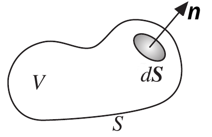
Figure 4. Control volume for conservation equations.
Vector \(n\) - pointing outward - is the normal vector to a small portion \(dS\) on the surface \(S\). Let us consider the total amount of an arbitrary property \(Φ\) (in units of the property itself) in the volume \(V\). The property can be energy, mass, heat or whatever, and let \(φ\) be the density of \(Φ\) in a small portion \(dV\) of the volume \(V\). \(Φ\), within volume \(V\), can change for a source of \(Φ\) within \(V\) or flux of \(Φ\) through the boundary. The latter can take place for fluid transport or in absence of fluid transport, for instance for heat conduction. Therefore, we can express the change over time of \(Φ\) through the relationship
$$\frac{d}{dt}\int_V\varphi dV=-\int_S Fds - \int_S \varphi vds + \int_V HdV (1).$$
where \(H\) is the source term, in units of \(Φ\) per unit time and unit volume, \(v\) is the component of velocity of transport along \(n\) and \(F\) is the flux of \(Φ\) in absence of fluid transport and is expressed in terms of \(Φ\) per unit time and surface S. The negative signs on the right hand side are justified by considering that an outward flux of \(Φ\) implies a negative rate of change within volume \(V\).
Eq.1 is a simplified form of Reynolds' transport theorem and is valid for any volume \(V\) even if the field is not continuous. Let us note that in calculating the integral we loose any information on the spatial variability within volume \(V\). Let us also note that \(φ\), \(F\), and \(H\) depend on the spatial coordinates \(x\), \(y\) and \(z\) as well as time \(t\). We do not explicitly indicate here the above dependencies to simplify notation.
Equation (1) lends itself to some considerations. For simplicity, let us assume that we apply it to the case of a tank collecting water from a known input and releasing output from a bottom discharge and let us assume that \(Φ\) is the water volume \(w\) in the reservoir and \(φ\) is water density that we indicate here with the symbol \(ρ\)(figure 5).
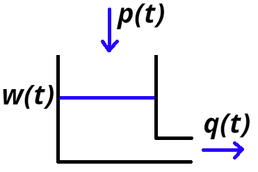
Figure 5. Control volume for conservation equations.
For simplicity we assume that there is no source term and only fluid transport. In such conditions, eq. 1 reduces to (let us to explicitly indicate dependence on time in this case)
$$\frac{d}{dt}w(t)=- \int_S \rho v(t)ds=p(t)-q(t) (2).$$
Eq(2) is a differential equation because we need here to describe change in storage. If we assume that there are no changes in storage, eq.2 would reduce to \(p(t)=q(t)\) which is an integral equation. the latter conclusion can be generalised: conservation equation are expressed in differential form for the need to describe the storage term.
Application in continuum mechanics
Let us now assume that the field of the property \(Φ\) is continuous, like for instance in classical fluid mechanics. If we are interested in describing the spatial and temporal variability of the system, given that we in principle loose any information on the internal distribution within volume \(V\), we then need to refer to a very small size of \(V\) itself, so that we do not loose much information on spatial variability when averaging over \(V\).
Then, we need to refer to the concept of "representative volume element" (RVE), which should be small enough to allow us to neglect the spatial variability of \(Φ\) within RVE. Given the existence of a suitable continuum length scale, we can rewrite eq. (1) above as a local partial differential equation. If we assume that the average value of \(Φ\) over V is differentiable, we can replace the surface integrals using Gauss' theorem to replace the integral over S with an integral over V:
$$-\int_S Fds-\int_s \varphi v ds = - \int_V \nabla (F+\varphi v) dV. (3)$$
Moreover, because the surface and volume are fixed in an inertial frame then the time derivative of the summed properties is equal to the sum of the local time derivatives:
$$\frac{d}{dt}\int_V \varphi dV = \int_V\frac{\partial \varphi}{\partial t}dV. (4)$$
Substituting eq. 3 and eq. 4 into eq. 1 yields:
$$\int_V \left[\frac{\partial \varphi}{\partial t} + \nabla (F+\varphi v)-H\right] dv=0. (5)$$
Because V is of arbitrary shape and size, eq. (5) can only be satisfied if the term in square brackets is zero everywhere, thus
$$\frac{\partial \varphi}{\partial t} + \nabla (F+\varphi v)-H =0. (6)$$
This is the general form of all conservation laws in continuum mechanics. If we assume \(F=0\) and \(H=0\) we obtain
$$\frac{\partial \varphi}{\partial t} + \nabla (\varphi v)=0. (7)$$
The above relationships, depending on the specific assumptions, deliver the concept underlying the development of Earth system models. Despite the apparently complicated mathematical treatment, application of conservation laws is in many cases simple. See, for instance, the example of the tank depicted in figure 5.
Uncertainty assessment for Earth system models
Uncertainty assessment for future predictions of the state of the Earth systems is essential for providing support to management strategies. Uncertainty is an essential information in project design. It has to be estimated by using an objective method and following the ethics of engineering, namely, by requiring honesty, impartiality, fairness, and equity, and hold paramount the safety, health, and welfare of the public. This is essential as design project is different from scientific investigation. Structures and infrastructures that interact with the Earth system may expose human communities at risk - think for instance of a bridge, or a dam. Therefore the design implies a responsibility that is bore by the engineer.
Such responsibility implies that uncertainty assessment must provide a reliable estimation of the errors that may be expected in design variables with respect to what may really happen. Uncertainty may be originated by several drivers including:
- Uncertainty in input variables and initial conditions;
- Uncertainty in model parameters;
- Inhability of the model to reproduce the underlying processes (model structural uncertainty).
Uncertainty is often estimated by using different models to determine the values of design variables, thus obtaining an envelope of responses. This technique provides an estimate of model output variability, but does not take into account the structural uncertainty of any single model. In other words, if the models are all similar and all wrong, we will obtain a narrow envelope that would not include the true value. Uncertainty assessment for environmental models is an active field of research.
State of the Earth system and perturbations
We live under the perception that the Earth system is naturally in equilibrium and that such equilibrium is perturbed by human impact. Actually, the Earth system is never in equilibrium, as it is continuously exposed to natural and human induced perturbations. It is an evolving system, that is permanently in transition. Example of transitional periods are the ice ages, the period after important volcanic eruptions or impact with asteroids and so forth. Human disturbances may interact with natural perturbations thus contributing to changes of state, that may be transitional or permanent.
Examples of natural disturbances are:
- Volcano Eruptions: emissions of hashes and dust from volcanic eruptions may cause extended pollution of the atmosphere and reduce the income of solar energy, thereby implying alteration of local and possibly global climate. Moreover, local, regional, and perhaps global extinctions may occur due to deposits of massive amounts of volcanic material and extended global cooling.
- Asteroid Impact: may cause the formation of large crateers, with high-pressure metamorphism in zone of impact, seismic energy release, vaporization of large amounts of surface and groundwater, frictional heating as impactor enters atmosphere, local to global extinction due to impact, alteration of the inclination of the terrestrial axis.
- Earthquake: may induce the release of dust, debris, and toxic gases.
- Cooling of the earth nucleous: Earth's interior has been gradually cooling for the entirety of its 4.5 billion-year history. It is a generally helpful pattern as the planet evolved into its current green paradise. Cooling of the interior is a natural process that in the long term weakens the magnetic field, thus inducing the same consequences as the geomagnetic reversal described below. Cooling of the Earth's core will lead to uninhabitability in millions or billions of years from now. Therefore, cooling leads to wonder how long life will last on the Earth.
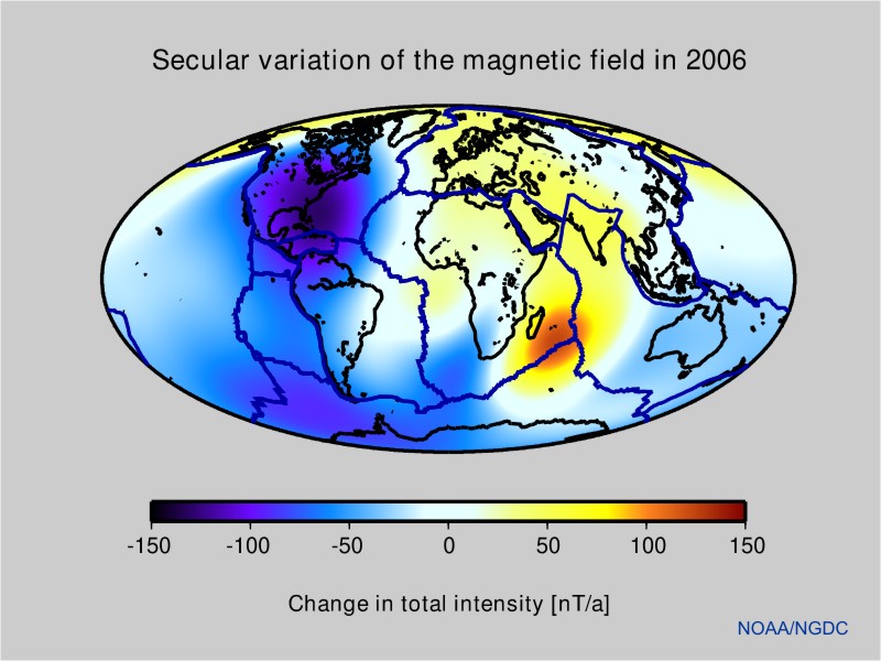
- Geomagnetic reversal: it is a change in a planet's magnetic field such that the positions of magnetic north and south are switched. Through its history, the Earth's field has alternated between periods of normal polarity, in which the predominant direction of the field was the same as in the present time, and reverse polarity, in which it was the opposite. These periods are called chrons. There have been at least 183 reversals over the last 83 million years (on average once every ~450,000 years). The latest, the Brunhes–Matuyama reversal, occurred 780,000 years ago. Some scientists think that geomagnetic reversals are not spontaneous processes but rather are triggered by external events that directly disrupt the flow in the Earth's core. The causes of the reversal are an active field of research. Some scientists hypothesises that reversals could provoke mass extinctions, as the Earth's magnetic field would be much weaker during reversals. Thus, high-energy particles trapped in the Van Allen radiation belt could be liberated and bombard the Earth. Also, some researchers argue that the atmosphere of Mars may have been eroded away by the solar wind because it had no longer magnetic field to protect it. The magnetic field also undergoes slow changes with a time scale of years. Accurate measurements of the magnetic field, provided by satellites and magnetic observatories, can be used to estimate the present changes in the field. Secular variations of the field are shown in Figure 7. It shows that the field strength is decreasing in most parts of the World. The strongest decrease is seen the Caribbean. But there are also areas of increasing field strength, such as in the Indian Ocean.
Examples of disturbances that can be natural and/or human induced are:
- Deforestation: loss of vegetation affects regional transpiration, water storage, and drainage patterns, thus implying an alteration of the distribution of water resources.
- Viral pandemic: causes widespread sickness and mortality among human species and therefore it is impacting the environment through disruption of conservation practices, increase of pullution and so forth.
- Climate change: leads to perturbations of the climate system that may cause the crossing of tipping points.
Natural and anthropogenic perturbations may resonate, therefore originating amplification of disturbances and risk. Understanding perturbations is a necessary requirement to avoid resonance and to design mitigation and adaptation policies.
Earth system sciences
Earth system sciences, or geosciences, are the sciences that study the Earth system for the sake of understanding the inherent dynamics and mitigate related risks. For the complexity of processes, and the numerous spheres of the Earth system, geosciences is articulated in several branches, including but not limited to:
- climate science,
- hydrology,
- biogeosciences,
- atmospheric sciences,
- ocean sciences,
- geology,
- tectonics,
and so forth. Geosciences also include space and planetary sciences. Research in geosciences is promoted by several international scientific associations, including the American Geophysical Union, the European Geosciences Union, the Japanese Geosciences Union, the AOGS, the International Union of Geodesy and Geophysics, and so forth.
Download the powerpoint presentation of this lecture
Last revised on Feb 26, 2024
- 3156 viste