
Stochastic models assume that the occurrence of waves can be assimilated to random events, namely, an event that cannot be described deterministically. Random events are unpredictable. However, they sometimes apparently follow patterns. These are indeed determined by a material cause, which in our case is determined by the law of physics, but an exact list of its forcings may be unknown or impossible to analytically specify.

Figure 1. Rolling a dice is a classical example of a random event (from Wikipedia)
To deal with random events and to carry out inference on them, it is necessary to associate them to numbers. This association creates the random variable, which is an association between a random event and a real (or integer, or complex) number. In our case, we treat the extreme wave as a random variable, which is the association between the event of a flood and a real number. Random variables can be discrete or continuous. In first case the number of outcomes is finite, while in the second case we need to deal with infinite possible outcomes.
The stochastic model is therefore called to provide an estimate for the extreme wave height treated as a random variable, by taking advantage of all the available information. To understand the essence and the possible structures of stochastic models we need to introduce some concepts of probability theory.
1.2.1. Basic concepts of probability theory Probability describes the likelihood of an event. Probability is quantified as a number between 0 and 1 (where 0 indicates impossibility and 1 indicates certainty). The higher the probability of an event, the higher the likelihood that the event will occur. Probability may be defined through the Kolmogorov axioms. Probability may be estimated through an objective analysis of experiments, or through belief. This subdivision originates two definitions of probability.
The frequentist definition is a standard interpretation of probability; it defines an event's probability as the limit of its relative frequency in a large number of trials. Such definition automatically satisfies Kolmogorov's axioms.
The Bayesian definition associates probability to a quantity that represents a state of knowledge, or a state of belief. Such definition may also satisfy Kolmogorov's axioms, although it is not a necessary condition.
Frequentist and Bayesian probabilities should not be seen as competing alternatives. In fact, the frequentist approach is useful when repeated experiment can be performed (like tossing a coin), while the Bayesian method is particularly advantageous when only a limited number of experiments, or no experiments at all, can be carried out. The Bayesian approach is particularly useful when a prior information is available, for instance by means of physical knowledge.
1.2.2. Probability distribution A probability distribution assigns a probability to a considered random event. To define a probability distribution, one needs to distinguish between discrete and continuous random variables. In the discrete case, one can easily assign a probability to each possible value, by means of intuition or by experiments. For example, when rolling a fair die, one easily gets that each of the six values 1 to 6 has equal probability that is equal to 1/6. One may get the same results by performing repeated experiments.
In the case a random variable takes real values, like for the river flow, probabilities can be nonzero only if they refer to intervals. To compute the probability that the outcome from a real random variable falls in a given interval, one needs to define the probability density. Let us suppose that a interval with length 2Δx is centered around a generic outcome x of the random variable X, from the extremes x-Δx and x+Δx. Now, let us suppose that repeated experiments are performed by extracting random outcomes from X. The frequency of those outcomes falling into the above interval can be computed as:
Fr(x-Δx;x+Δx) = N(x)/N,
where N(x) is the number of outcomes falling into the interval and N is the total number of experiments. We can define the probability density of x, f(x), as:
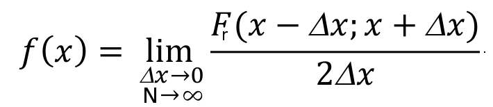
If an analytical function exists for f(x), this is the probability density function, which is also called probability distribution function, and is indicated with the symbol "pdf". If the probability density is integrated over the domain of X, from its lower extreme up to the considered value x, one obtains the probability that the random value is not higher than x, namely, the probability of not exceedance. The integral of the probability density can be computed for each value of X and is indicated as "cumulative probability". By integrating f(x), if the integral exists, one obtains the cumulative probability distribution F(X), which is often indicated with the symbol "CDF".

Figure 5. The probability function p(S) specifies the probability distribution for the sum S of counts from two dice. For example, the figure shows that p(11) = 1/18. p(S) allows the computation of probabilities of events such as P(S > 9) = 1/12 + 1/18 + 1/36 = 1/6, and all other probabilities in the distribution.
Example: the Gaussian or normal distribution The Gaussian or Normal distribution, although not much used for the direct modeling of wave extremes, is a very interesting example of probability distribution. I am quoting from Wikipedia:
"In probability theory, the normal (or Gaussian) distribution is a very common continuous probability distribution. Normal distributions are important in statistics and are often used in the natural and social sciences to represent real-valued random variables whose distributions are not known. The normal distribution is useful because of the central limit theorem. In its most general form, under some conditions (which include finite variance), it states that averages of random variables independently drawn from independent distributions converge in distribution to the normal, that is, become normally distributed when the number of random variables is sufficiently large. Physical quantities that are expected to be the sum of many independent processes (such as measurement errors) often have distributions that are nearly normal. Moreover, many results and methods (such as propagation of uncertainty and least squares parameter fitting) can be derived analytically in explicit form when the relevant variables are normally distributed."
The probability density function of the Gaussian Distribution reads as (from Wikipedia):

where μ is the mean of the distribution and σ is its standard deviation.
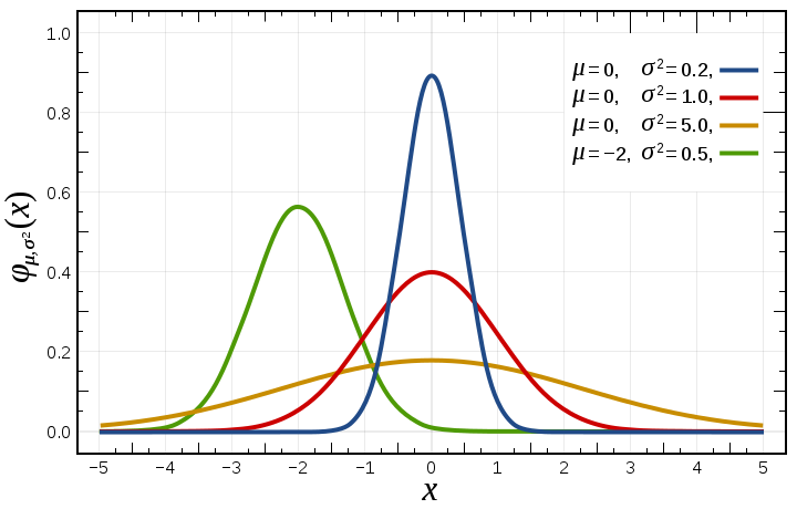
Figure 6. Probability density function for the normal distribution (from Wikipedia)
The above introduction to probability theory suggests the use of a widely applied method to estimate the extreme wave height, that is, to estimate a probability distribution to describe the frequency of occurrence of extreme data. In fact, we already realized that the return period, which is an essential information that conditions extreme wave estimation, can be related to the frequency of occurrence and therefore the probability of occurrence. It follows that one can associate to a return period the corresponding probability of occurrence, which can be in turn related to the corresponding river flow through a suitable probability distribution. In fact, the return period is the inverse of the expected number of occurrences in a year. For example, a 10-year wave has a 1/10=0.1 or 10% chance of being exceeded in any one year and a 50-year wave has a 0.02 or 2% chance of being exceeded in any one year. Therefore, if we fix the return period we can derive the related extreme wave by inverting its probability distribution. Furthermore, probability theory provides us with tools to infer the uncertainty of the estimate. For the sake of brevity we are not discussing how to estimate uncertainty when applying the annual maxima method.
In coastal engineering, the probability distribution of peak wave height may be inferred by studying the frequency of occurrence of annual maxima. Basically, from the available record of observations one extracts the annual maximum value for each year and the statistical inference is carried out over the sample of annual maxima. According to this procedure, the annual maximum return period is the average interval between years containing a wave height of at least the assigned magnitude.
The annual maxima method is conditioned by the assumption that the random process governing the annual maximum value is independent and stationary. Independence means that each outcome of annual maximum flow is independent of the other outcomes. This assumption is generally satisfied in practice because it is unlikely that the occurrences of annual maxima are produced by dependent events (although dependence may happen if long term persistence is present, or the storm season crosses the months of December and January). Stationarity basically means that the frequency properties of the extreme flows do not change along time (please note that the rigorous definition of stationarity is given here.
Stationarity is much debated today, because several researchers question its validity in the presence of environmental change, and in particular climate change. In some publications the validity of concepts of probability and return period is questioned as well. However, the technical usefulness of stationarity as a working hypothesis is still unquestionable. For more information on the above debate on stationarity, see here and here.
Several different probability distributions can be used to infer the probability of the annual maximum values. The most widely used is perhaps the Gumbel distribution, which reads as: F(x) = e-e-(x-μ)/β where μ is the mode, the median is  and the mean is given by
  where
where  is the Euler–Mascheroni constant
  The standard deviation of the Gumbel distribution is
  Once a sufficiently long record of waves is available, the statistics of the distribution (i.e., the mean and the standard deviations) can be equated to the corresponding sample statistics and therefore the distribution parameters can be easily estimated.
The Gumbel distribution was proposed by Emil Julius Gumbel in 1958.
Example of application - Annual maxima method and Gumbel distribution Let us suppose that a record of 10 annual maxima is available, including the following observations: 239.0; 271.1; 370.0; 486.0; 384.0; 408.0; 148.0; 335.0; 315.0; 508.0 One is required to estimate the 5-year return period design variable.
The mean of the observations is 346.41 and the standard deviation is 110.08. Therefore, one obtains that β=85.80 and μ=296.88. The probability of not exceedance corresponding to the return period of 5 years is P(Q)=(T-1)/T=4/5=0.8 By inverting the Gumbel distribution one obtains: X(T)= -β(log(-log(P(X))))+μ or X(T)= -β(log(log(T/(T-1))))+μ Therefore, one obtains: X(5)=425.56
1.3.1. Is the Gumbel distribution fitting the data well? When one applied a probability distribution to describe the frequency of occurrence of random events, the question should be raised on the capability of the probability distribution to provide a good fit. To check the reliability of the distribution, statistical tests can be applied. The most used test for verifying probability distributions is the Kolmogorov–Smirnov test. Please refer to the given link for a description of the test.

Figure 7. Illustration of the Kolmogorov–Smirnov statistic. Here, X is a generic random variable that can take both positive and negative values. Red line is CDF, blue line is an ECDF, and the black arrow is the K–S statistic (from Wikipedia. Please see the description of the Kolmogorov–Smirnov test on Wikipedia for mode details).
1.3.2. Data requirements for the annual maxima method The annual maxima method therefore requires the availability of a sufficiently long series of annual maxima. The larger the return period, the larger the sample size of the observed data should be. An empirical rule suggests not to extrapolate the Gumbel distribution beyond a return period that is twice the size of the observed sample. One should also take into account that the Gumbel distribution generally overestimates when extrapolated.
1.3.3. Alternative probability distributions for the annual maxima method There are several alternatives to the use of the Gumbel distribution within the annual maxima method. The most used probability distributions, besides the Gumbel, are the Frechet Distribution and the GEV distribution, which includes the Gumbel and Frechet distributions as special cases.
The annual maxima method presents the disadvantage of selecting and using for the statistical inference one value only per each year. Therefore, potentially significant events, occurred in the same year, may be discarded in the analysis. To resolve this problem, the peak-over-threshold method (POT) can be applied, which analyses all the peak values exceeding a given limit. Different probability distributions are usually applied to fit the obtained sample. More details are provided here.
The Generalized Pareto Distribution (GPD) is the most used probability model for threshold excesses and the shape parameter is determining the tail behavior of the distribution. Buoy measurements are the trustworthy data source and can be used in the analysis. The GPD distribution is characterized by three parameters: location, scale and shape. Location corresponds to the value of the threshold. If the shape and location are both zero, the GPD is equivalent to the exponential distribution. Packages are available in R to estimate the GPD parameters with several different estimators. More details on the GPD distribution are given here.
Another vital aspect is the seasonality constraints in climate data. It was suggested that the year should be split-up into months or other sensible period by Carter and Challenor (1981). When dealing with coastal management, analysis of flooding risk and the design of off-shore structures depend on the seasonal or monthly characteristic in the return value calculation (Minguez et al., 2010). This homogeneity can be ensured by separation into carefully selected seasons
Peak Over Threshold (POT) method for wave heights was used and it was fitted to GPD (Mackay et al., 2010). Annual Maxima (AM) approach solves immediately some problems of the initial distribution method, however main difficulty of this method is, dealing with lack of enough data for distribution fitting (Soares and Scotto, 2004). The AM method is not appropriate, because less number of annual maxima data points will not provide good estimates (Soares and Scotto, 2001). Various methods can be used for the threshold selection. There is a trade-off between bias of the estimated extreme design variables (low threshold) and variance due to the limited number of data used for estimating the GPD parameters (high threshold).
Mean residual life plot was suggested by Stansell (2004) to select the specific cut-off value. This graphical diagnostic technique is based on a characteristic property of the GPD distribution. In fact, if the GPD is a valid model for excesses over some threshold u0, then it is valid for excesses over all thresholds u > u0. Furthermore, for u > u0 it can be proved that the expected value of the difference given the given random variable and the threshold value, which can be estimated by the sample mean of the threshold excesses, is a linear function of u. This results provides a ready to use diagnostic technique which can be applied prior to the actual model fitting.
An alternative approach is to assess the stability of parameter estimates. Hence, this sensitivity analysis for model fitting is performed across a range of different threshold values.
Finally, diagnostic checks can be applied once the GPD distribution has been estimated. They are discussed in the exercise titled "Estimation of extreme wave height" (see here).
References
Carter, D. J. T., & Challenor, P. G. (1981). Estimating return values of environmental parameters. Quarterly Journal of the Royal Meteorological Society, 107(451), 259-266.
Mínguez, R., Menéndez, M., Méndez, F. J., & Losada, I. J. (2010). Sensitivity analysis of time-dependent generalized extreme value models for ocean climate variables. Advances in water resources, 33(8), 833-845.
Mackay, E. B., Challenor, P. G., & Bahaj, A. S. (2010). On the use of discrete seasonal and directional models for the estimation of extreme wave conditions. Ocean Engineering, 37(5), 425-442.
Soares, C. G., & Scotto, M. (2001). Modelling uncertainty in long-term predictions of significant wave height. Ocean Engineering, 28(3), 329-342.
Soares, C. G., & Scotto, M. G. (2004). Application of the r largest-order statistics for long-term predictions of significant wave height. Coastal Engineering, 51(5), 387-394.
Stansell, P. (2004). Distributions of freak wave heights measured in the North Sea. Applied Ocean Research, 26(1), 35-48.
The video of this lecture (Part 2)
Last modified on May 2nd, 2017
- 52 views