

Earth system models usually are parametric models, namely, they include parameters. When discussing about rainfall-runoff modeling it was emphasized that parameters are numeric factors in the model equations that can assume different values therefore making the model flexible. Indeed, the parameter can be defined as a measurable factor in the constitutive equations of the model, that can assume different values therefore making the shape of the equation flexible while maintaining its structure. Parameters usually assume fixed values, but they may also depend on time, or the state of the system. Parameters are introduced in order to be able to adapt the model and optimize its performances in simulating a real world phenomenon. In order to apply the model, parameters needs to be estimated (or calibrated, or optimized, and we say that the model is calibrated, parameterized, optimized).
Parameter calibration can be carried out by following two main avenues, namely, (a) by optimizing model performances or (b) through expert knowledge.
The most frequently used calibration procedure is through the optimization of model performances, which is carried out by comparing observed and simulated data. An example of such comparison for the calibration of a rainfall runoff model is reported in Figure 1 (Brath et al., 2004).
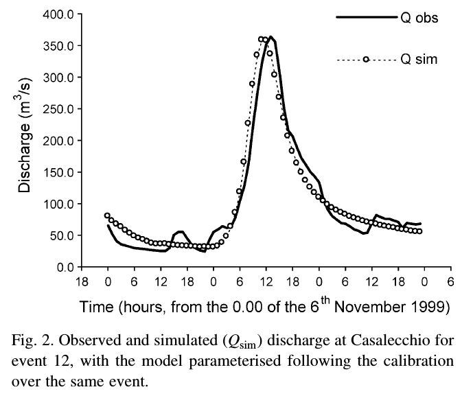
Figure 1. Calibration of a rainfall-runoff model through comparison between observed and simulated data (from Brath et al., 2004).
The search for the best parameter values can be carried by following a trial and error procedure, which was the most used approach in the past. Accordingly, one makes an initial guess of the parameter value and runs the model therefore obtaining simulated data values that are visually compared with the corresponding observations. If the simulation is not satisfactory the parameter value is changed and the model is ran again. The simulation is repeated until a satisfactory solution is obtained. The trial and error procedure presents the advantage of allowing a full control by the user of the process, so that the user gains confidence with the model and a full perception of the model strengths and weaknesses. The drawback is that the procedure takes a substantial amount of time, and may become impossible to carry out with increasing number of parameters and therefore increasing number of possible solutions. The complexity of model calibration when several parameters are involved is the reason why simple models, with few parameters, were mainly used in the past.
With the advent in the late eighties and nineties of the past century of personal computer, which quickly provided unprecedented computational means, the researchers devised automatic procedures for parameter calibration. The idea is to make the trial and error procedure automatic, therefore designing algorithms to automatically make subsequent trials of model parameters. The ability to perform millions of trials in a relatively short time gave to researchers the capability of quickly calibrating complex models including several parameters. The application of this automatic procedure requires the identification of a numerical criteria to evaluate the goodness of model performances, which is necessarily to be carried out by the algorithm automatically. Such numerical criteria were identified by devising objective functions or loss functions, which are functions mapping values of one or more variables onto a real number intuitively representing model performances. Therefore, for the case of rainfall-runoff modeling the objective function is in charge of deciphering the goodness of a simulated hydrograph or a simulated characteristic of the hydrograph, like the peak flow, the hydrograph volume etc.
The literature proposed several objectives functions to be used in hydrology. The most used is the sum of squares or least squares, which can be written as
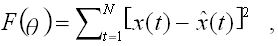
where θ is the vector of parameters (which may reduce to one value), x(t) is the observed variable at time t and the hat symbol indicates the corresponding value simulated by the model, while N is the number of observations over which the sum of squares is computed. The lower the F(θ) value, the better the model performances. Therefore, one seeks the θ value that minimizes F(θ). The idea behind the sum of squares is very simple, that is, to minimize the sum of the squared model errors, which are squared to avoid compensation between positive and negative errors. The appropriateness of the sum of squares objective function for model calibration is also confirmed by statistical reasoning which proves its consistency and unbiasedness under certain assumptions, which however are rarely met in hydrological applications. The sum of squares objective function is actually biased when applied to most hydrological models. For rainfall-runoff models, for instance, it is intuitive that it give more emphasis to the fit of the higher flows. In fact, by squaring the error more weight is given to the larger errors, which are typically experienced in the simulation of the high flows. The practical consequence is that the sum of squares objective function is not the most appropriate solution for optimizing the fit of low flows.
An objective function that is largely used, which has similar behaviors as the sum of squares, is the Nash-Sutcliffe efficiency, which is given by
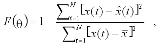
where x is the mean of the observed data. The Nash-Sutcliffe efficiency varies from -∞ to 1, where 1 indicates perfect model performances. Conversely, an efficiency of 0 indicates a model that has the same predictive performances as the mean of the observed data. The Nash-Sutcliffe efficiency has the advantage of allowing a comparison between the performances of different models applied to simulate different phenomena. When the Nash-Sutcliffe efficiency is applied to quantify the performances of rainfall-runoff models, a rule of thumb suggests that values lower than 0.5 indicate poor predictive capabilities, but a refined evaluation is of course to be carried out case by case.
When the simulation of the low flows is to be optimized, one may adopt the sum of the absolute errors, which is given by
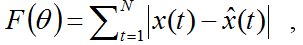
with the same meaning of the symbols. If one wants to put even more emphasis on the low flows, the sum of the absolute relative error may be used, namely,
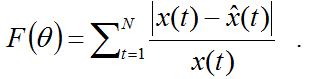
The latter should be used with caution. In fact, if the observed value tends to zero, then the objective function is inflated by giving enormous weight to the related observations. Therefore the sum of absolute relative errors should not be used when observations are tending to zero.
The literature proposes several other objective functions. Some of them have well known statistical properties, others are not statistically based and therefore may be biased or inconsistent. However, unbiasedness and consistency are not necessary features. They testify that the model parameters provide the best simulation of all the observations. However, if the interest of the user is the good simulation of selected observations, or selected features of the simulated variables, then consistency and unbiasedness may not be a high priority requirement. Therefore, creativity may be used in the definition of the objective function, by considering the purpose of the application and the design goals, therefore fitting the model for purpose.
Parameter values can be guessed by expert knowledge, therefore avoiding the need for observed data. This solution is used in ungauged basins. For instance, the user may decide to transfer the parameter values from a neighboring or similar catchment, or may decide to base the calibration on his/her own experience. For instance, when calibrating the linear reservoir rainfall-runoff model one may decide to set the bottom discharge time constant by equating it to the time of concentration of the catchment, which in turn might be estimated by using an empirical relationship.
Expert calibration if of course potentially subjected to a relevant uncertainty, but it might be a very good solution to resolve real world applications.
One should always beware that calibration trains the model with respect to selected hydrological conditions, which are those resembled by the observed data. When applied to so-called "out of sample situations", namely, when applied to hydrological conditions that significantly differ from those which calibration referred to, the model may provide less satisfactory performances with respect to what emerged from calibration. This is a significant practical problem, which may negatively impact the reliability of engineering design. The problem is alleviated when the model is calibrated by using a very extended sample, but this is rarely the case in hydrology, where the sample size of observed data is usually limited. Therefore, it is recommended that the model is tested to check its performances in real world applications, after calibration and before using it in practice. Such testing procedure is called validation. The term validation is well known in hydrology and environmental modelling and is commonly used to indicate a procedure aimed at analysing the performance of simulation and/or forecasting models. In the scientific context, the term validation has a broader meaning including any process that has the goal of verifying the ability of a procedure to accomplish a given scope.
A simple and intuitive way of performing validation for a hydrological model is to use the so-called "split-sample" procedure. The observed data are divided into two groups: one group is used for calibration and the other group is used to test the model by emulating a real world application, namely, by performing a out-of-sample application. Then, the procedure may be repeated by inverting the group of data used for calibration and validation, therefore obtaining two validation tests. If the sample is sufficiently large, it can be split in three pieces and so forth. The similarity or dissimilarity of the parameter values in different calibration procedures provides an indication of the reliability of the estimates. Before finally applying the model, it is advisable to finally get the parameter values to be used in practice by performing a calibration by using the whole data sample, to reduce the uncertainty of the parameter estimates as much as possible.
Validation is always appropriate in engineering design, in view of the uncertainty affecting hydrological models. The literature also suggested more elaborated validation procedures, like for instance the cross-validation.
Brath, A., Montanari, A., Moretti G., Assessing the effect on flood frequency of land use change via hydrological simulation (with uncertainty), Journal of Hydrology, Vol. 324, 141-153, 2006.
Last modified on October 9, 2021
- 1661 views