
Coastal hydrodynamics and morphodynamics studies the circulation of sea water in the proximity of the shoreline, as well as the associated erosive process, sediment transport and any other process that contributes to shaping the morphology of coast and beach. The above processes evolve along different spatial and temporal scales, according to complex dynamics that are driven by several forcings and impacted by several environmental behaviors. The latter include the wave and wind regimes, the geometry of the embayment, the presence of coastal protections, the shape and geology of the coast, the sediment size of the beach and many others.
The morphodynamic approach to beaches and coastal systems recognizes the range of interactions among the above processes occurring across the full environmental system. It consider the related two-ways (positive and negative) feedbacks and coevolution which determine the dynamic equilibrium of the coastline. The morphodynamic approach to coastal modeling, design and management originated during the sixties of the 20th century, at the Coastal Studies Institute (CSI) at Louisiana State University (Short and Jackson, 2013). In what follows we will concentrate on the study of the beach, which may be defined as a gradual landward transition to the shoreface, which is usually composed by loose particles. The beach extends from the low-water mark to the highest high-water mark. Because the backshore is often considerably flatter in appearance than the foreshore, which slopes clearly down towards the sea, it is also often referred to as a beach platform. To set up the basis for the analysis of beach hydrodynamics and morphodinamics, it is necessary to recall basic concepts of waves motion and beach structure. The basic nomenclature of sea waves is explained by Figure 1.

Figure 1. Basic nomenclature of a sea wave. By NOAA - http://oceanservice.noaa.gov/education/kits/currents/media/supp_cur03a.html, Public Domain, https://commons.wikimedia.org/w/index.php?curid=50074693.
The nomenclature of beaches is introduced here. Additional terms will be introduced in what follows.
Figure 2 shows the typical structure of a beach formed by loose particles. In the offshore area, waves do not interact with the seafloor and therefore there is no significant mass movement. The shaping of the sea bottom is mainly driven by tectonic forcing with igneous activity having a strong role (activity related to the displacement of heated rocks at the fluid state). Initial structural and volcanic creations are slightly modified by deposition of sediments originated by deep sea currents. These processes evolve according to a time scale of thousands of years.
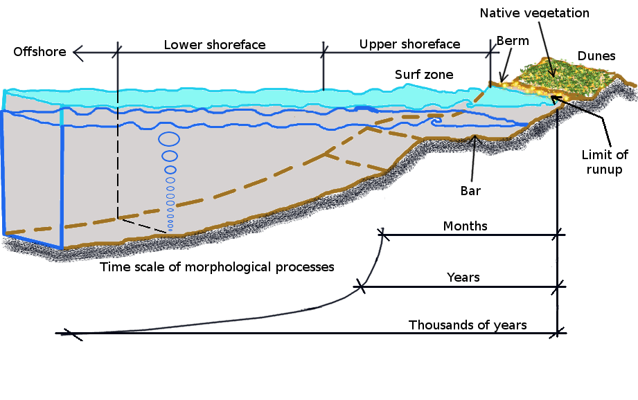
Figure 2. Structure of a generic beach
In the proximity of the shoreline, the depth of water decreases and waves start to interact with the seafloor. This zone is called the "lower shoreface" and is characterised by increasing amplitude of waves. In fact, with decreasing water depth, the conservation of the energy flux conveyed by waves requires the waves increasing their amplitude therefore originating the "shoaling" (see Figure 3).
Figure 3. Conservation of energy flux in decreasing sea depth nearshore originates process of shoaling, which takes place in the so-called "shoaling zone". By Régis Lachaume - own artwork, CC BY-SA 3.0, https://commons.wikimedia.org/w/index.php?curid=3799016
If the water depth keep decreasing, the waves become increasingly higher. Moreover, the lower part of the wave is slower with respect to the upper part, because of the friction with the seafloor. The combination of the above forcing and motion dynamics brings the wave at a critical level where it collapses therefore originating turbulence, so that a large amounts of wave energy is transformed into turbulent kinetic energy. The zone after the wave breaking is called the surf zone. After breaking in the surf zone, the waves (now reduced in height) continue to move in, and they run up onto the sloping front of the beach, forming an uprush of water called swash.Turbulence causes a relevant mass of water to move towards the shoreline and back, along the upper shoreface, therefore originating a shoreward current which is compensated by a counter-current along the bottom. A significant transport of sediments is associated to the currents, which shapes the upper shoreface. As the waves approach the shoreline, the above mass movement causes the alternative covering and exposure of what is called the swash zone, which evolves according to time scales ranging from months to years.
Where the wave break, therefore approximately at the boundary between the shoaling zone and the swash zone, a sandbars may form, because the sand carried by the moving bottom current is deposited where the current reaches the wave break. Sandbars consist mainly of sand or gravel, depending on the material available along the coast. The sides of the sandbar fall gently away. The basin between a sandbar and the shore zone is called the runnel or swale. Other longshore bars may lie further offshore, representing the break point of even larger waves, or the break point at low tide. Longshore bars can also form at river mouths by the deposition of freshwater sediments.
At the upper limit of the swash zone, on the beach there is very often a bank of sand or a gravel ridge parallel to the shoreline and a few tens of centimetres high, known as the berm. On its landward side there is often a shallow runnel. The berm is formed by material transported by the breaking waves that is thrown beyond the average level of the sea. The coarse-grained material that can no longer be washed away by the backwash remains behind. The location and size of the berm is subject to seasonal changes. For example, a winter bern that has been thrown up by storm surges in winter is usually much more prominent and higher up the beach than berms formed by summer high tides. The farthest point inland that is reached by storm surges is bounded by a belt of dunes, where floods can form a dune cliff. The dune if often populated by native vegetation that is able to capture the low amount of freshwater flowing into the dune sand. See Figure 4, 5 and 6.
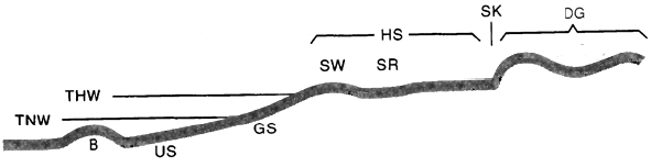
Figure 4. Diagram of a flat coast littoral series. Key: B: bar, TNW: average low tide, THW: average high tide, US: shoreface; GS: foreshore, SW: berm, SR: runnel, HS: backshore, DG: dune belt, SK: dune cliff. By --HylgeriaK 12:19, 3. Mär. 2009 (CET) - Own work (Original text: selbst erstellt), Public Domain, https://commons.wikimedia.org/w/index.php?curid=17854014

Figure 5. The berm: where the gravel is no longer washed back into the sea by the backwash. The Gulf of Salerno: Salerno (on the right), the Coast of Amalfi and the Lattari Mountains. By No machine-readable author provided. Giaros assumed (based on copyright claims). [GFDL (http://www.gnu.org/copyleft/fdl.html), CC-BY-SA-3.0 (http://creativecommons.org/licenses/by-sa/3.0/) or CC BY-SA 2.5-2.0-1.0 (http://creativecommons.org/licenses/by-sa/2.5-2.0-1.0)], via Wikimedia Commons.

Figure 6. Start of the dune belt by the sand cliff. Quinta do Lago beach (Praia da Quinta do Lago). Algarve, Portugal. CC BY-SA 2.0, https://commons.wikimedia.org/w/index.php?curid=168142
Sea waves are originated by winds and associated friction over the water surface, sea currents or exceptional movements of the earth's surface associated to earthquakes (in this case they are called "tsunami waves"). We will focus on wind waves which originate from wind blowing over the sea surface and can travel thousands of kilometers before reaching land. The restoring force is provided by gravity, and so they are often referred to as surface gravity waves. The size of wind waves ranges from that of small ripples to over 30 meters high. In particular, in some cases rogue waves (also called freak waves, monster waves, episodic waves, killer waves, extreme waves, and abnormal waves) have been observed. These are defined as a single wave whose amplitude is more than twice the mean of the largest third of waves in a wave record. Rogue waves appear suddenly and are often unpredictable, and cannot be simulated with the linear theory. The mechanism leading to their formation is still largely unknown, but they are probably originated by the superimposition of wind waves and waves originated by sea currents. Rogue waves are dangerous even to large ships.
After the wind ceases to blow, wind waves are called swells. More generally, a swell is series of waves that have been generated by distant weather systems, where wind blows for a duration of time over a fetch of water.
The dynamics of wind waves is characterized by the presence of randomness, which determines their height, duration, and shape with limited predictability. As such, waves and their behaviors can be described as a stochastic process, in combination with the physics governing their generation, growth, propagation and decay. The physics of waves is governed by the following main drivers:
- Wind speed and duration. Wind is the sources of energy for wind waves and therefore regulates the energy transfer from wind to waves.
- The uninterrupted distance of open water over which the wind blows without significant change in direction (called the fetch).
- Width of area affected by fetch.
- Sea depth.
In open sea and ocean, the movement of the waves is given by a shift of forms rather than mass of water. If fact, waves are the expression of a shift of energy rather than mass. Only after breaking a significant movement of mass of water occurs back and forth in the swash zone. In the open sea the movement of mass is negligible and occurs only in the proximity of the surface, as an effect of the Stokes drift. In fact, particles in linear plane waves of one wavelength in deep water move not plainly up and down but in circular orbits that are slightly shifted forward. These orbits move forward above and backward below, with respect to the wave propagation direction (See Figure 7).
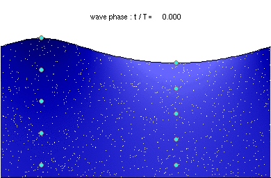
Figure 7. Water particle motion in a linear plane wave. By Kraaiennest - Own work, GFDL, https://commons.wikimedia.org/w/index.php?curid=3374567
The size of a single transversal sea wave (namely, a wave that is oscillating perpendicularly to the direction of propagation) and its propagation is characterized by the following main behaviors:
- Wave amplitude.
- Wave length.
- Wave period or frequency.
- Wave direction.
In open ocean, it is convenient to refer to plane waves, namely, waves whose wavefronts (surfaces of constant phase) are infinite parallel planes. Design variables for off-shore and inshore structures are mostly derived by assessing the average and extreme value of the above wave behaviors, and in particular the wave amplitude, frequency and direction. In order to better understand the design principles for the above structures it is useful to recall the basic concept of sea wave mechanics, which are summarized here. Monitoring and assessment of wave forcing is described here.
Breaking waves close to the shoreline combine with along shore currents to originate the transport of beach sediments. Displacement of sediment may take place at the local level or may be extended over long distances in the along-shore and cross-shore directions. Along-shore sediment transport is responsible of long term variations. Cross-shore erosion and deposition is responsible of rapid shocks during extreme events. Sediment movement is the primary cause of beach erosion and replenishment, and is impacted by weather, geometry and geology of the shoreline and human impact. At some coastal sites the rate of transport can be as large as several millions of cubic meters of sand per year. Sediment transport may occur with different behaviors in the different seasons.
Sediment transport may occur in the form of bed-load and suspended transport. It may be measured by using several different techniques. More details are given in the Coastal Engineering Manual of the US Corps of Engineers, which is available here.
To identify signatures of along-shore sediment transport provides useful indications to understand beach morphodynamics. Such qualitative features usually provide indications about net sediment transport, which is the result of the difference between right-directed and left-directed transport. Sand entrapment by structures like groyns and other infrastructures may provide useful hints to identify the dominant direction and magnitude of transport. A long-shore decrease of the size of sediment grains may also provide indications on the direction of transport, as well as the identification of unique minerals in the sediments. Tracers can also be used, in the form of unique minerals or colored sediments. Repeated observation of forms evolution and surveys can be used to determine sediment transport quantitatively.
In engineering applications, the longshore sediment transport may be expressed as the volume transport rate Ql. It may be expressed in cubic meters per day or year. It may also be given in immersed weight transport rate, which can be easily related to the volume transport rate once the mass density of the sediment grains and water are known. Table 1 provides an overview of the longshore transport rate in selected coasts in the US.

Table 1. Longshore transport rates in selected US coasts. From Coastal Engineering Manual of the US Corps of Engineers.
The first formulas for estimating along-shore sediment transport were derived by relating the flux of sediments to deepwater wave energy. A frequently used approach is provided by the so-called CERC formula or energy-flux method. CERC is the acronym of the Coastal Engineering Research Center of the US. The concept underlying the formula was first proposed in the early 20th century. The CERC relationship, that we illustrate here below, was first proposed in 1970. For more details one look here.
Let us assume that the total longshore sediment transport rate is related to the longshore component of the energy flux which is generated by waves that approach the shore at an angle. We indicate with the symbol Eb the wave energy density per unit horizontal area at the breaker line. It can be computed by referring to the linear wave theory and the case of a periodic single plane wave, by adopting two alternative solutions, leading to the same result.
The first solution is obtained by equating Eb to the mean wave energy density per unit horizontal area averaged over a wave cycle. Let us recall that, in general, the wave energy is given by the sum of the kinetic and potential energy density, integrated over the depth of the fluid layer. Potential and kinetic energy oscillate during the wave cycle by compensating each other, so that the total energy is conserved and is equal to the mean wave energy. The potential mean energy density per unit horizontal area averaged over a wave cycle for a periodic wave can be computed through the relationship (see also here)

where η and db are the elevation of the wave surface and the sea depth with respect to the mean water level, respectively, Hb and a are the wave height and amplitude, respectively, and ρ and g are mass density of sea water and gravity, respectively. Note that η is varying in time and therefore the average is computed over a complete wave cycle. Note also that the energy is per unit horizontal area as the above computation computes potential energy by considering mass density of water instead of mass. Mass density is mass per unit volume and the resulting energy is integrated along the vertical direction, so what we obtain is indeed energy per unit horizontal area. Finally, note that the above relationship is dimensionally consistent, by taking into account that Eb is energy per unit area.
It can be proved (see here for more details) that according to the linear wave theory the mean kinetic energy density per unit horizontal area is equal to the above mean potential density per unit horizontal area. Therefore the total energy density of the wave at the breaker line per unit horizontal area is given by
Eb = (ρg Hb2)/8.
The same result can be achieved by considering that the kinetic energy of the periodic single plane wave is null when the wave reaches the upper and lower elevation. The distribution of kinetic and potential energy along the time of propagation of a periodic wave is pictured in this graph which is embedded in this page explaining the distribution of wave energy. Therefore the total energy at the breaker line is equal to the potential energy of the wave at the upper and lower elevation which is given by the relationship

As waves propagate, their energy is transported. The energy transport velocity is the group velocity. As a result, the wave energy flux, through a vertical plane of unit width perpendicular to the wave propagation direction, is equal to (see here for more details)
Ebw=EbCbg
where Cbg is the wave group velocity at the breaker line. The latter can be estimated through the relationship
Cbg= (gdb)0.5=(g Hb/k)0.5
where k = Hb/db is the breaker index.
Then, we define the potential longshore sediment transport rate Pl as the immersed weight of sediments per unit time that may be potentially transported for given sea and shoreline conditions provided enough material is available to be transported. It may be estimated through the relationship
Pl = Ebw sinαb cosαb = Eb Cbg sinαb cosαb
where αb is the acute angle between the breaker line and the coast line. On the one hand, multiplication by sinα leads to obtaining the longshore component of the energy flow; on the other hand, multiplication by cosα allows to compute the flux in the direction of wave advance per unit length of beach. In terms of longshore transport the most impacting situation then occurs when α=45°.
Note that the above relationship is dimensionally consistent and that an empirical correction of the estimate will be introduced below for taking into account that the underlying assumption of sediment transport given by energy flux may be not satisfied in real world applications.
With simple transformations of trigonometric functions Pl can be computed as
Pl = 1/2 Eb Cbg sin2αb.
The immersed and "actual" weight transport rate can be obtained by multiplying Pl by an empirical coefficient, namely,
Il = K Pl
where K is a dimensionless parameter with 0 ≤ K ≤ 1. The above relationship can be converted to a volume transport rate:
Ql = K Pl/((ρs-ρ)g(1 - n))
where ρs, ρ and n are the mass density of sediment grains, mass density of water and sediment porosity, respectively. For the K coefficient empirical values are suggested by the literature. Calibration of K is advisable for practical applications. The above presented formula is often called the "CERC formula".
Once the longshore transport is known, sediment balance can be imposed along elementary along shore spatial steps to compute the rate of beach erosion or accretion (see Figure 8).
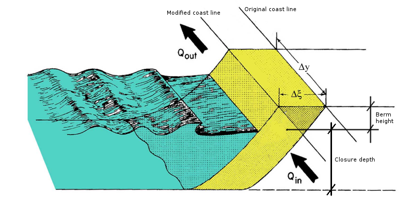
Figure 8. Computation of beach profile under the effect of longshore sediment transport. Source: tutorial of prof. Musumeci, University of Catania
Computation can be performed by using the 1-line model, which is based on the frequent observation that the beach profile maintains an average shape that is characteristic of that particular coast. Beach features like slope and closure depth are preserved in the long term. Although seasonal changes in wave climate cause the position of the shoreline to move in a cyclical manner, the departure from the characteristic shape are relatively small. Therefore the beach profile responds to wave action by translating back and forth during erosion and accretion, under the assumption that the beach profile moves parallel to itself. If the profile shape does not change, the observed contour line can be used to describe change in the beach plan shape and volume as the beach erodes and accretes. This contour line may be conveniently taken as the readily observed shoreline, and the model is therefore called the "shoreline change" or "shoreline response" model. Sometimes the terminology "one-line" model, a shortening of the phrase "one-contour line" model is used with reference to the single contour line. The model may be applied to discrete portions of beach, where the beach profile does not change in each portion, but can change at larger scale.
A second assumption is that sand is transported alongshore between two well-defined limiting elevations on the profile in the cross-shore direction. The landward limit is located at the top of the active berm and the seaward limit is located where no significant depth changes occur, the so-called depth of closure. Restriction of profile movement between these two limits provides the simplest way to specify the perimeter of a beach cross-sectional area by which changes in volume, leading to shoreline change, can be computed.
For many decades longshore sediment transport has been considered the dominant process to determine beach morphodynamics. The focus on cross-shore sediment transport is more recent. Cross-shore sediment transport includes both offshore and onshore transport. The former dominates when heavy storms occur, while the latter is the dominant process in mild conditions. Due to its development in short time scale, offshore transport turns out to be more easily predictable. This is an opportunity as offshore transport is indeed more interesting for engineering applications, as it is significantly impacting the morphology of beaches and land.
Cross-shore sediment transport is relevant to several coastal engineering problems, including beach and dune development, design of beach nourishment projects, shoreline response to sea level rise, seasonal variations of shoreline positions, which can be relevant, and seaward scour of shore-parallel structures. Figure 9, 10, 11 and 12 show the evolution of the beach profile corresponding to a shock originated by a severe storm, sea level raise, beach nourishment and the construction of a seawall, respectively.
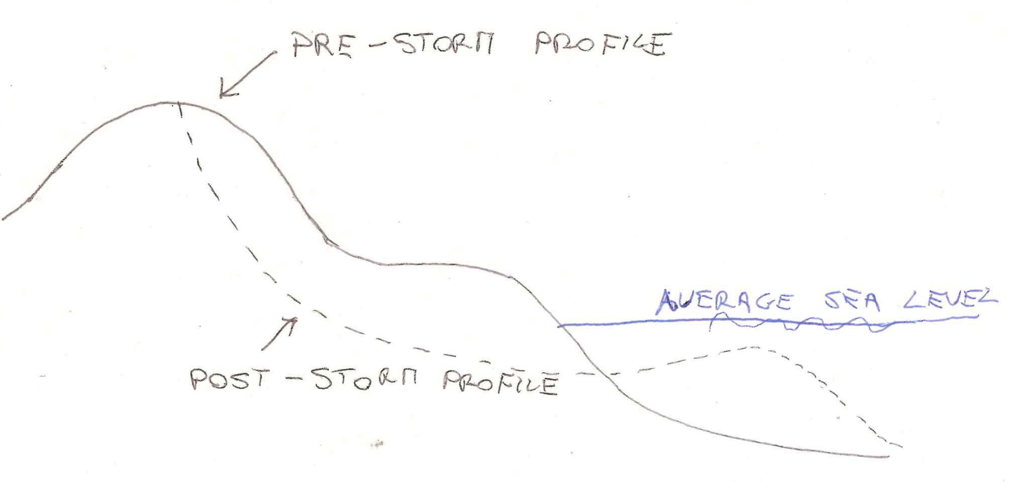
Figure 9. Evolution of beach profile after erosion triggered by an extreme event.
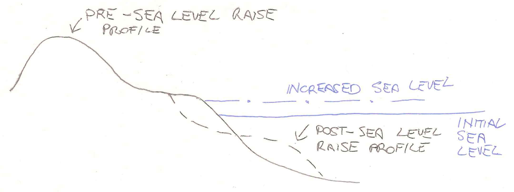
Figure 10. Evolution of beach profile triggered by sea level raise.
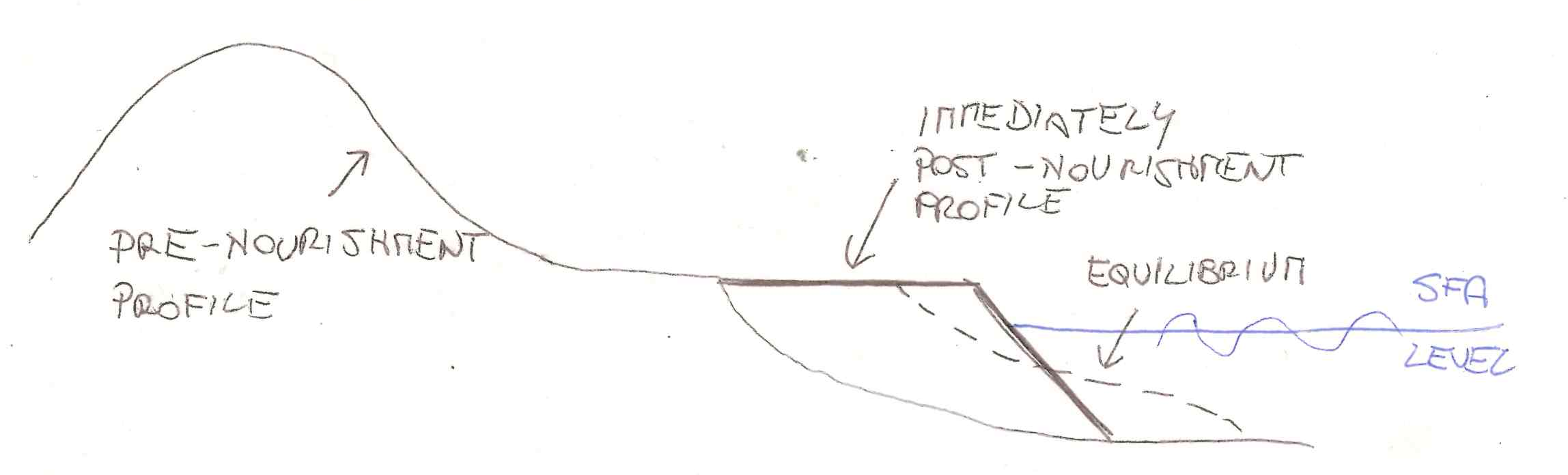
Figure 11. Evolution of beach profile triggered by beach nourishment.
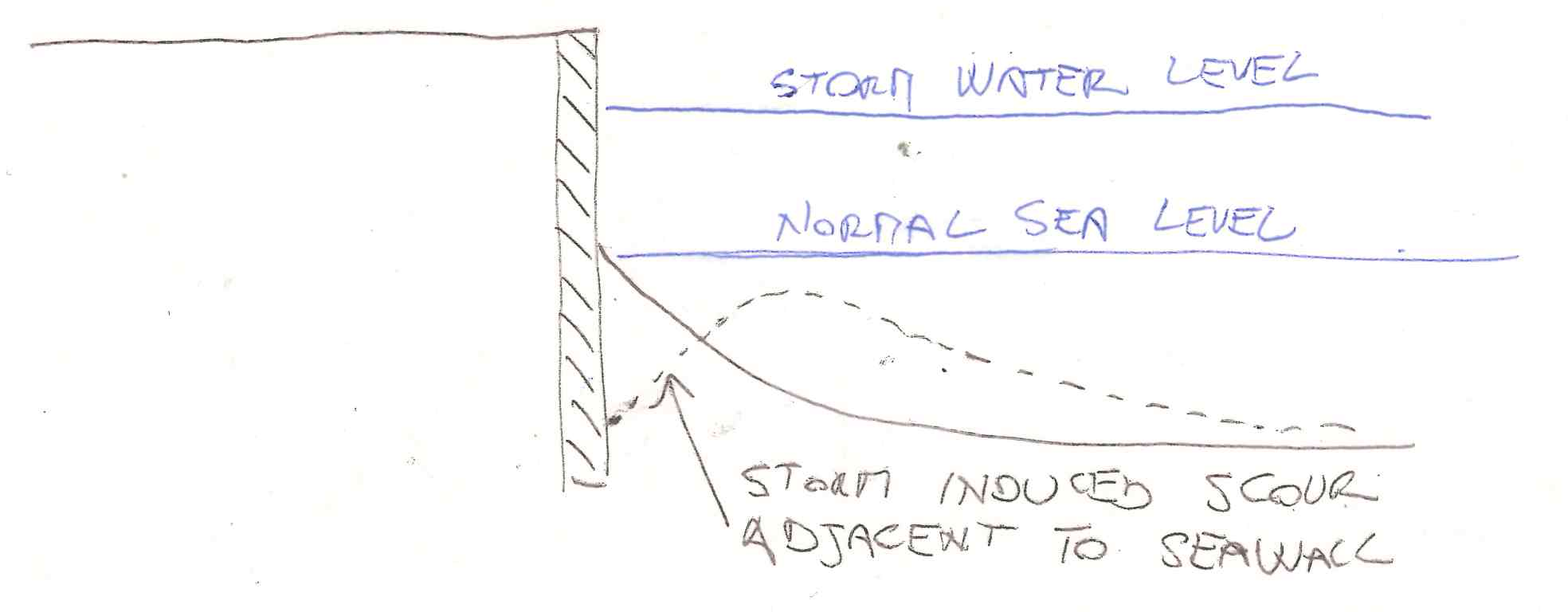
Figure 12. Evolution of beach profile triggered by the construction of a seawall.
Depending on the sea conditions and related sediment transport components, the beach may be prone to erosion or deposition. The latter takes place when destructive forces prevail on constructive ones, therefore originating the formation of a bar usually located where waves break. Deposition occurs when constructive forces prevail, therefore originating the berm at the upper limit of the swash zone. Several real world observations proved that the berm typically originates for the mild action of waves during the summer season, while the bar originates when destructive forces prevail during storms in the winter season.
The above erosion and deposition processes are excellently exemplified in this video, which shows the result of a laboratory experiment that is presented here. In particular, the description of the hydraulic conditions during the video read as: "The first part of the video is 2 hours of 12.4 cm waves with a period of 1.3 seconds. These steep waves produce large destructive forces on the beach slope. The beaches response is to flatten out and does this by slowly eroding the berm (the dry portion of the beach). The eroded sediment is then transported offshore and built up as sand bars. Sand continues to erode, flattening the beach until the wave machine is stopped. The wave period is then changed and the height kept roughly the same producing longer, more gradual waves. These waves lasted 3 hours and 15 minutes and were 12.1 cm high at 3.1 seconds. These longer period waves produced more constructive forces which result in the sand from the bar being transported in a ridge and runnel system on shore. The sand from the bar is transported back onto the beach, producing accretion of the eroded shoreline until the beach face is back to the original wider, steeper profile."
Several criteria have been proposed to determine empirically when erosion prevails on deposition. The Sunamura and Horikawa criteria says that equilibrium occurs when the following relationship is satisfied:
H0/L0 = K tan(β)-0.27 (D50/L0)0.67
where H0 and L0 are wave height and length in deepwater, K is a constant, β is the beach slope and D50 is the grain diameter of the beach particles that 50% of a sample's mass is smaller than. When the left hand side of the above formula prevails over the right hand side erosion originates, while deposition occurs when the right hand side dominates. Laboratory experiments indicated values for K around 4, while real world observations suggest K = 9.
Several research efforts have been spent to understand and represent in detail with mathematical models cross-shore sediment transport, for the purpose of predicting the evolution of the beach profile. The process results from a combination of constructive (originating deposition) and destructive (originating erosion) forces, which are discussed here below.
A first constructive force is originated by the interpretation of water particle velocities provided by several wave theories. Accordingly, it can be proved that the time average of the water particle velocity is null, while the average bottom shear stress is positive and directed onshore, therefore originating the transport of sediment towards the shoreline.
A second constructive force originates within the bottom boundary layer, causing a net mean velocity in the direction of propagating water waves. This streaming motion was first observed in the laboratory and it is due to the local transfer of momentum associated with energy losses by friction. A contribution is also given by suspended sediment transport and turbulence. Depending on the behaviour of waves, it can be either constructive or destructive.
A first destructive force is given by gravity. A second contribution is given by seaward currents in the swash zone. A third contribution is originated by seaward currents originated by transfer of momentum flux from the wave to the water column in the surf zone. Finally, wind originate a forcing that can be either constructive or destructive.
To provide an interpretation of the evolution of the beach profile, researchers attempted to derive relationships for the prediction of the cross-shore sediment transport in the different zones of the shoreline (surf zone, swash zone, etc.). The inherent nature of these relationships is empirical, although some of them were derived by physical considerations. We will not describe these relationships here. An extensive discussion is provided in the Chapter III of the Coastal Engineering Manual of the US Army Corps of Engineers.
Once sediment transport is determined, the evolution of the beach profile can be modelled by applying Exner's equation, namely:
∂ h/∂ t = - ∂ q/∂ x
where h is bed aggradation, upward positive, q is the flux of crossing shore sediments expressed in cubic meters over time per unit longshore extension and x is the coordinate in the cross shore direction. Boundary conditions are imposed by annihilating the sediment transport at the upper limit of the swash zone and the boundary between near shore and open ocean.
Engineers, US Army Corps Of. "Coastal engineering manual." Engineer Manual 1110 (2002): 2-1100. Available online at http://www.publications.usace.army.mil/USACE-Publications/Engineer-Manuals/?udt_43544_param_page=4.
Short A.D., and Jackson D.W.T. (2013) Beach Morphodynamics. In: John F. Shroder (ed.) Treatise on Geomorphology, Volume 10, pp. 106-129. San Diego: Academic Press.
Sunamura, Tsuguo, and Kiyoshi Horikawa. "Two dimensional beach transformation due to waves." Coastal Engineering 1974. 1975. 920-938.
The Powerpoint presentation of this lecture
Last modified on March 6, 2019
- 697 views